This article was published as a part of the Data Science Blogathon.
What are Activation Functions?
Activation functions are mathematical functions in an artificial neuron that decides whether it should be activated,i.e, turned on or not.
An artificial neuron takes a linear combination of the inputs from the neurons of the previous layer and applies the activation function to generate the final output of that activation function.
It decides whether that particular neuron has a role for a given set of inputs(neuron should be ON or OFF) and if the neuron is activated(ON), how much role it has in the output(magnitude value of the output of activation function)
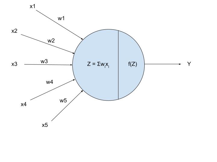
Fig 1: Artificial Neuron, Source: Author
In the above figure,f(Z) showcases the activation functions.
Here, xi is the inputs and wi are the weights corresponding to them. The node takes the weighted sum and feeds it to the activation functions to get the final output Y.
Y = f(Z)
Y = Activation Function(Weights Sum of Inputs)
An activation function serves 2 purposes :
1. Determines whether a neuron must be activated or not and how much say that neuron has in the overall neural network.
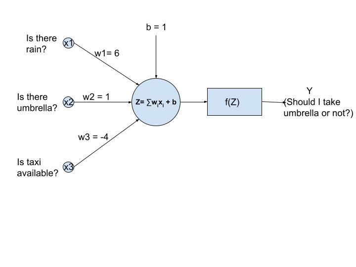
Fig 2: Artificial Neural Network for solving a simple problem, Source: Author
The above network is an artificial neural network that’s used to analyze/find the probability if someone should take an umbrella or not based on 3 inputs
a.x1 = Is there rain? b. x2=Is there an umbrella? c. x3=Is a taxi available?
There are also 3 arbitrary chosen weights for each input(both excitatory and inhibitory weights)
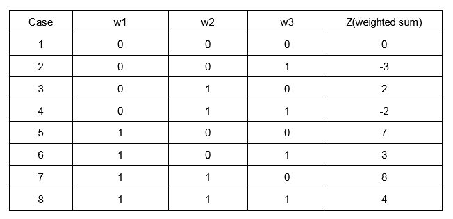
As you can see Z is the weighted sum of the inputs for the current set of weights which gives magnitude output. We need to see if the umbrella should be taken based on a Yes(0) or No(0) as the output from the neural network. This is where an activation function comes into the picture. Since We need a Yes or No,i.e,1 or 0, a step function should be used as the activation function.
Equation
Image Source: https://atomurl.net/math/
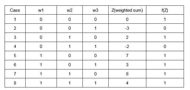
So the activation functions gave a clear answer to the problem statement.
2. Introduces non-linearity into the neural networks which are mandatory for solving real-world problems.
A network without activation function would cause a linear relationship between the input(s) and the output(s),i.e,f(Z) = Z , so will be only as good as a linear regression model, not for solving any complex models.
In an artificial neural network, the weights and biases of the neural network are updated using backpropagation after finding the gradients to calculate the errors. Since the gradient of the linear relationship would be 1, no updation will be happening to the weights and biases.
The choice of activation function has a critical impact on the accuracy and performance of the model. It is important to choose the most apt activation function for a particular application.
What are the Different Types?
Sigmoid
Equation:
Image Source: https://atomurl.net/math/
Graph:
Image Source: https://www.transum.org/Maths/Activity/Graph/Desmos.asp
Function Input Range : (- ∞,∞)
Function Output Range : (0,1)
Working: The function takes in any real values between —∞ and -∞ as the input and outputs values between 0 and 1. More the input value close to ∞ , the closer it will be to +1 and similarly the more the input value is close to –∞ , the closer it will be to 0.
Application: Sigmoid activation function is used for neural networks where we need to find the probability as the output(since its output is between 0 and 1). It is used for binary classification problems.
Advantages:
1. It normalizes the input values and bounds them between 0 and 1, enabling clear predictions.
2. The function is a continuous function and also differentiable. So there is no discontinuity/jump in gradient calculation which means it works well with backpropagation.
Disadvantages:
1. The gradient of the function is less for the higher values(closer to ∞) and for the lower values(closer to –∞). So for these values, the vanishing gradient problem arises,i.e, the error gradient calculation results in a smaller value than intended and the learning process slows down for these 2 cases.
2. When sigmoid is used for output layer multi-class classification problems, the sum of output probabilities may not be equal to 1 , so to rectify this softmax is used for multi-class classification problems.
3. It is not zero centred, so learning for negative inputs is less compared with learning for positive inputs.
4. It is highly computationally intensive since it has to calculate exponential.
Python Code:
import numpy as np
def sigmoid(z) :
exp_fn = np.exp(-z)
fn = 1/(1+ exp_fn)
return(fn)
Softmax
Graph:
Image Source : https://www.transum.org/Maths/Activity/Graph/Desmos.asp
Function Input Range : (- ∞,∞)
Function Output Range : (0,1)
Working: The function normalizes the outputs for each class between 0 and 1, adds the normalized sum for each class. The output for a particular class is its normalized output divided by the total normalized sum.
Application: The softmax activation function is used for multi-class classification. It will calculate the probabilities of each class. Let’s say there is a 16 class classification problem solved using a CNN. The softmax activation function will be used at the output/last layer.
When an input image is fed into the CNN, after extracting features using hidden layers, the output softmax function will give probabilities of each class. The sum of probabilities will be 1(,i.e,100%).
Advantages:
1. Sum of probabilities is 1, perfect for multi-class classification
2. The function is a continuous function and also differentiable. So there is no discontinuity in gradient calculation which means it works well with backpropagation.
Disadvantages:
1. It can be used as output/last layer only.
2. It is the most computational intensive activation function that even hardware accelerators are used sometimes just to calculate softmax function output.
Python Code:
import numpy as np
def softmax(z) :
exp_fn = np.exp(z)
sum_exp_fn = np.sum(np.exp(z))
fn = exp_fn/sum_exp_fn
return(fn)
Hyperbolic Tangent (tanh)
Equation:
Image Source: https://atomurl.net/math/
Graph:
Image Source: https://www.transum.org/Maths/Activity/Graph/Desmos.asp
Function Input Range : (- ∞,∞)
Function Output Range : (-1,1)
Working: The function takes in any real values between —∞ and -∞ as the input and outputs values between -1 and 1 as the output. More the input value close to ∞ , the closer it will be to +1 and similarly the more the input value is close to –∞ , closer it will be to -1.
Application: It has the same applications as sigmoid since it is very similar to it. The only difference between them is that for negative inputs, in the case of sigmoid the output closes on to 0, here for tanh, the output closes on to -1. It is used for binary classification problems.
Advantages:
1. It is a zero centred function, which means it works well/learns well equally for positive and negative inputs.
2. Converges faster than sigmoid due to symmetry.
3. It also acts as a dropout layer in hidden layers(since 0 is an output).
Disadvantages:
1. Similar to sigmoid, it also faces the vanishing gradient problem at largely positive inputs(output close to +1) and largely negative inputs(output close to -1).
2. It is highly computationally intensive
Python Code:
import numpy as np
def tanh(z) :
exp_fn_1 = np.exp(z)
exp_fn_2 = np.exp(-z)
fn = (exp_fn_1-exp_fn_2)/(exp_fn_1+exp_fn_2)
return(fn)
ReLU(Rectified Linear Unit)
Equation: f(Z) = max(0,Z)
Image Source :https://atomurl.net/math/
Graph:
Image Source: https://www.researchgate.net/figure/ReLU-activation-function_fig7_333411007
Function Input Range : (- ∞,∞)
Function Output Range : (0,∞)
Working : For all positive values,the output is same as input.For negative values,the output is 0,i.e,the neuron is dead.The gradient(derivative) of ReLU is 1 for inputs greater than 0 and equal to 0 for negative inputs.
Application: ReLU is used for CNN, Natural Language Processing, Pattern Recognition models which require deep neural networks.When you are in a dilemma about which activation function to use, use ReLU.
Advantages:
1. It has a constant derivative, so can be used for the neural networks which suffer from vanishing and exploding gradient problems.
2. It is the best activation function for CNNs because it is most efficient for extracting features or for pattern recognition.
3. It is faster to compute(both function, for forwarding propagation and its gradient, for backpropagation). So training with networks having ReLU activation function would consume less time when compared to the same network with other activation functions like sigmoid or swish.
4. It can act as a dropout layer,i.e, deactivates the neuron completely if the input to it is 0.
Disadvantages:
1. It is not differentiable at 0, so continuous output requiring problems cannot use ReLU as an activation function.
2. The Dying ReLU problem: When the input to neuron is a negative value, its gradient is 0, so, during backpropagation, no learning occurs for this input. To eliminate this, Leaky ReLU is used.
Python Code:
import numpy as np
def ReLU(z) :
fn =np.max(0,z)
return(fn)
Leaky ReLU(LReLU)
Equation: f(Z) = max(0.01Z,Z)
Image Source : https://atomurl.net/math/
Graph:
Image Source: https://www.i2tutorials.com/explain-step-threshold-and-leaky-relu-activation-functions/
Function Input Range : (- ∞,∞)
Function Output Range : (-∞,∞)
Working: For all positive values, the output is the same as the input. For negative values, the output is 0.01 times the input.
The gradient(derivative) of ReLU is 1 for inputs greater than 0 and equal to 0.01 for negative inputs.
To eliminate the ‘dying ReLU’ issue, Leaky ReLU activation is used. In this, the function is initialized with a small value for all inputs less than 0, so that learning happens(backpropagation works) when negative inputs are fed to it.
Application: It is used for CNN, NLP, Pattern Recognition models which requires deep neural networks.
Advantages:
1. It solves the ‘Dying ReLU’ problem by initializing the function with an arbitrary value for negative inputs. So for negative inputs, some learning occurs
2. Increase inaccuracy of the model when compared with the model having ReLU.
Disadvantages:
1. The gradient for the whole range of negative inputs is 0.01 which is a very small value. So even though backpropagation and thus learning occurs,it is very slow. This is solved using PReLU where the slope can be modified.
Python Code:
import numpy as np
def LReLU(z) :
fn =np.max(0.01z,z)
return(fn)
Parametric ReLU(PReLU)
Equation: f(Z) = max(αZ,Z)
Graph:
Image Source : https://paperswithcode.com/method/prelu
Function Input Range : (- ∞,∞)
Function Output Range : (-∞,∞)
Working: For all positive values, the output is the same as the input. For negative values, the output is the parameter α times the input.
The gradient(derivative) of ReLU is 1 for inputs greater than 0 and equal to α for negative inputs.
The slope/gradient can be modified by the user as per desire to get the desired accuracy and to get faster convergence.
Application: It is used for CNN, NLP, Pattern Recognition models which requires deep neural networks.
Advantages:
1. Increase inaccuracy of the model and faster convergence when compared with the model having LReLU and ReLU.
Disadvantages:
1. The user has to manually modify the parameter α by trial and error.
2. For different applications, different α would be required, finding which is time-consuming
3. For every negative input, the gradient remains the same irrespective of the magnitude. This implies during backpropagation, learning occurs equally for the whole range of negative inputs.
Python Code:
import numpy as np
def PReLU(z,α) :
fn =np.max(αz,z)
return(fn)
Exponential Linear Unit(ELU)
Equation:
Image Source: https://ml-cheatsheet.readthedocs.io/en/latest/activation_functions.html#elu
Graph :
Image Source: https://blog.paperspace.com/vanishing-gradients-activation-function/
Function Input Range : (- ∞,∞)
Function Output Range : (-α,∞)
Working: This function overcomes the disadvantages of ReLU and other ReLU variants. It takes in real values from – ∞ to ∞. For positive inputs, the output is the same as input and has a linear relationship. For negative inputs, it depends on 2 parameters, the first one is the input and the second one is the parameter.
Application: It is used for CNN, NLP, Pattern Recognition models which requires deep neural networks.
Advantages:
1. Increase inaccuracy of the model compared with the model having LReLU and ReLU.
2. It is the fastest converging ReLU variant.
Disadvantages:
1. The user has to manually modify the parameter α by trial and error.
2. It is computationally intensive due to the exponential in the calculation.
Python Code :
import numpy as np
def ELU(z,α) :
if(z>0 ) :
    fn = z
  else :
fn = α * (np.exp(z) - 1)
return(fn)
Scaled Exponential Linear Unit(SELU)
Equation:
Image Source: https://stats.stackexchange.com/questions/284642/what-is-the-backpropagation-formula-for-selu-activation-function
Graph :
Image Source : https://mlfromscratch.com/activation-functions-explained/
Function Input Range : (- ∞,∞)
Function Output Range : (- ∞,∞)
Working: When the input is positive, the output is λ times the input and for negative inputs, the output is λ times alpha times the exponential of input subtracted by 1.
Application: Sigmoid activation function is used for neural networks where we need to find the probability as the output(since its output is between 0 and 1). It is used for multi-class classification.
Advantages:
1. Vanishing and the Exploding gradient is non-existent for this activation function.
2. Faster convergence of the neural network.
3. It is a self normalizing activation function,i.e, mean becomes 0 and variance 1.
4. It can be used in very complex neural networks.
Disadvantages:
1. It is a highly computationally intensive function, might need special hardware accelerators for implementation.
Python Code:
import numpy as np
def ELU(z,α) :
if(z>0 ) :
fn = λ * z
else :
fn = λ*α * (np.exp(z) - 1)
return(fn)
9. Step Function
Equation:
Image Source: https://www.transum.org/Maths/Activity/Graph/Desmos.asp
Graph:
Image Source: https://en.wikibooks.org/wiki/Artificial_Neural_Networks/Activation_Functions
Function Input Range : (- ∞,∞)
Function Output Range : True(1) or False(0)
Working: It takes in all real values as input. For positive values, the output is 1 and for every negative value, the output is 0.
Application: Step activation is used for very simple binary classification problems(Yes/No problems) as illustrated at the beginning of this article.
Advantages:
1. Very simple function and uses almost nil computational resources.
Disadvantages:
1. It is not differentiable at 0. So zero gradients won’t backpropagate to update the weights.
2. Extremely limited application(merely binary classification).
Python Code:
import numpy as np
def step(z) :
  if(z>0 || z ==0) :
    fn=1
  else :
    fn =0
  return(fn)
Swish
Equation : f(Z) = Z * sigmoid(Z)
Graph:
Image Source: https://www.transum.org/Maths/Activity/Graph/Desmos.asp
Function Input Range : (- ∞,∞)
Function Output Range : (1/e,∞)
Working: For positive inputs, the output linearly increases with the input. For negative inputs, as the input closes on to, the output increases initially with the linear part(input z term). At larger values of the input, the sigmoid function becomes dominant and the output closes on to a constant value.
Application: It was developed by Google Brain Team to replace the most commonly used, yet not so perfect ReLU.It is used for the same applications as ReLU.
Advantages:
1. It helps to achieve higher accuracy for models than ReLU.
2. It has non-monotonic property for negative inputs. For every ReLU and ReLU variant, all are monotonic throughout for input less than 0.
3. It is a continuous function unlike ReLU and other variants which has a discontinuity at zero input.
Disadvantages:
1. It is highly computationally intensive
Python Code:
import numpy as np
def swish(z) :
exp_fn = np.exp(-z)
fn = x/(1+ exp_fn)
return(fn)
Sinusoidal
Equation: f(Z) = sin(Z), – ∞<Z<∞
Graph:
Image Source: https://www.geogebra.org/m/RvzVjyKr
Function Input Range : (- ∞,∞)
Function Output Range : [-1,1]
Working: It takes in values between – ∞ and ∞ calculates the sine of that. The output periodically oscillates in the range [-1,1].
Application: This function is used for training deep Fourier neural networks.
Advantages:
1. The studies for using sine function as an activation function for commonly used neural networks are ongoing. One of the studies showed that using them resulted in faster convergence of the model and more accuracy for a particular classification task. In future, we might see lots of applications using the sine function as an activation function.
Reference Paper: https://openreview.net/pdf?id=Sks3zF9eg
Disadvantages:
1. For increasing inputs, the output periodically increases and decreases and oscillates between +1 and -1. So it has a very specific application,i.e, for deep Fourier neural networks. Other networks cannot use this function.
Python Code:
import numpy as np
def sinusoidal(z) :
fn = np.sin(z)
return(fn)
Linear
Equation : f(Z) = Z
Graph:
Image Source : https://www.transum.org/Maths/Activity/Graph/Desmos.asp
Function Input Range: (- ∞,∞)
Function Output Range: (- ∞,∞)
Working: The output will be the same as the input.
Application: Linear Activation function is used for regression(univariate) problems.For instance, for calculating the price of a house when the area of the house is given, this activation function is used.
Advantages:
1. Large range of values can be obtained in the output, with no constraint.
2. The most simple activation function, no computational cost for implementation in the processor.
3. No room for exploding or vanishing gradient issues.
Disadvantages:
1. The derivative of this function is a constant. So backpropagation will not work(if there is an error in prediction since the gradient is constant, no dependence of error on the input, so it will not be reflected) with this function, so no learning happens for the neural network.
2. If there are multiple layers in the network, it will be only as good as a single layer neural network since the output is exactly the same as the input.
Python Code:
import numpy as np
def linear(z) :
fn = z
return(fn)
Where to use and which type of Activation Functions?
1. For regression problems(Only 1 neuron, multiple inputs, real-world outputs), a linear activation function must be used.
2. For multi-class classification problems, use Softmax at the output layer
3. For multi-label and binary classification problems, use the Sigmoid activation function.
4. Sigmoid and hyperbolic tangent activation functions must be never used in the hidden layers as they can lead to vanishing gradients.
5. For networks where unnecessary neurons need to turn OFF, use ReLU as the activation function because it also works as a dropout layer. In case there is confusion about which activation function, use ReLU.It is used in most CNN problems.
6. For deep neural networks having greater than 40 layers, use the swish activation function.
Hope you liked my article on activation functions? Share in the comments below. Read the latest blogs here.
The media shown in this article is not owned by Analytics Vidhya and are used at the Author’s discretion.


