This article was published as a part of the Data Science Blogathon.
Introduction
In this article, we are going to analyze the Amplitude Envelopes of different music genre tracks. This post is inspired by Valerio Valerdo’s work. I strongly advise you to visit his YouTube channel to see his incredible work in the field of Audio Machine Learning and Deep Learning.
Tools Used:
- Python
- Librosa
- One 30-second audio sample from each of five distinct music genres (Classical, Blues, Reggae, Rock, and Jazz) from the GTZAN dataset
What does the Amplitude Envelope of Audio Mean?
Amplitude Envelope: The amplitude envelope is a time-domain audio feature extracted from the raw audio waveform that refers to fluctuations in the amplitude of a sound over time and is an essential attribute since it influences our auditory perception of timbre. This is an important sound attribute because it allows us to swiftly detect and distinguish sounds. The maximum amplitude values among all samples in each frame make up the signal’s Amplitude Envelope which provides a rough estimation of loudness. This feature has been extensively used for onset detection and music genre classification. It is, however, more sensitive to outliers than the RMS energy audio feature, hence it is often less preferable to the RMS audio feature.
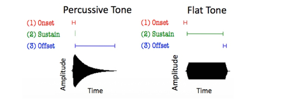
In one of its investigations, The MAPLE lab looked into two forms of amplitude envelopes: percussive and flat amplitude envelopes (see the diagram below). In percussive envelopes, an abrupt onset is followed by a quick exponential decay. This amplitude envelope is present in a variety of impact sounds, including slamming doors, hitting a drum, and so on. Flat amplitude envelopes, on the other hand, feature an abrupt onset, an extended sustain period, and an abrupt offset. These synthetic sounds are often used in several technological devices, including the dial tone on a phone call. Flat tones are also commonly used in experimental contexts because their qualitative qualities are easier to manipulate and control, although tones with a slope are more difficult to manipulate and control.
Furthermore, the usage of percussive vs. flat tones was found to have varied effects in various research disciplines. In a memory association exercise (including associations of melodic sequences and various home objects), participants remembered 60% more of the sequence-object correlations when percussive tone sequences were used instead of flat sequences. As a result, using sounds with different amplitude envelopes can make a big difference.

From the above diagram, it can be inferred that the percussive tones have no sustain with decay, whereas the flat tones are characterized by an indefinite sustain duration with abrupt offset.
Now, let’s explore the Amplitude Envelope using the librosa library.
Visualise the Amplitude Envelope of Different Music Genre Tracks
First, we’ll install librosa and import all of the required dependencies before loading the audio files.
Step 1: Install and import all the necessary dependencies
!pip install librosa
#importing all the necessary libraries

from IPython.display import Audio

import librosa

import librosa.display

import numpy as np

import matplotlib.pyplot as plt

%matplotlib inline
Step 2: Load the audio files
#load audio files
classical_music_file = "/content/drive/MyDrive/trytheseaudios/classical.00000.wav"
blues_music_file = "/content/drive/MyDrive/trytheseaudios/blues.00000.wav"
reggae_music_file = "/content/drive/MyDrive/trytheseaudios/reggae.00000.wav"
rock_music_file = "/content/drive/MyDrive/trytheseaudios/rock.00000.wav"
jazz_music_file = "/content/drive/MyDrive/trytheseaudios/jazz.00000.wav"
Next, we will load the audio files as a floating-point time series.
classical, sr = librosa.load(classical_music_file)
blues, _ = librosa.load(blues_music_file)
reggae, _ = librosa.load(reggae_music_file)
rock, _ = librosa.load(rock_music_file)
jazz, _ = librosa.load(jazz_music_file)
Following that, the duration of a single sample and the entire audio signal under examination will be computed. For demonstration purposes, I merely calculated it for the classical signal; similarly, we can compute for different audio signals from various genres.
Step 3: Compute the duration of a single sample and the entire audio signal under examination
sample_duration_classical = 1/sr
duration_of_classical_signal = sample_duration_classical * len(classical)
print(f"Duration of one sample is : {sample_duration_classical : .6f} seconds")
print(f"Duration of the audio signal is: {duration_of_classical_signal : .6f} seconds")
output: Duration of one sample is : 0.000045 seconds
Duration of the audio signal is: 30.013333 seconds
Step 4: Visualize different music genre track waveforms
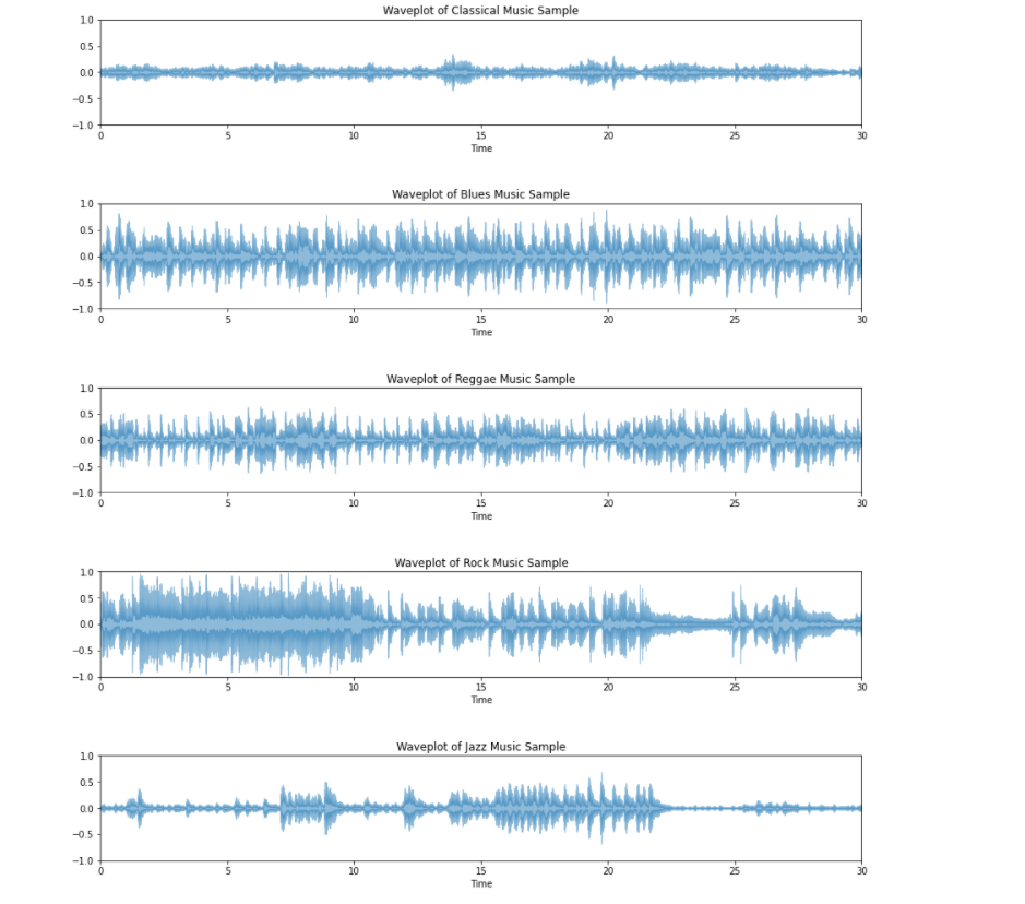
Let’s visualize the waveforms now!
#visualizing the waveforms
plt.figure(figsize=(15, 17))
plt.subplot(5,1,1)
librosa.display.waveplot(classical, alpha=0.5)
plt.title("Waveplot of Classical Music Sample")
plt.ylim(-1,1)
plt.subplot(5,1,2)
librosa.display.waveplot(blues, alpha=0.5)
plt.title("Waveplot of Blues Music Sample")
plt.ylim(-1,1)
plt.subplot(5,1,3)
librosa.display.waveplot(reggae, alpha=0.5)
plt.title("Waveplot of Reggae Music Sample")
plt.ylim(-1,1)
plt.subplot(5,1,4)
librosa.display.waveplot(rock, alpha=0.5)
plt.title("Waveplot of Rock Music Sample")
plt.ylim(-1,1)
plt.subplot(5,1,5)
librosa.display.waveplot(jazz, alpha=0.5)
plt.title("Waveplot of Jazz Music Sample")
plt.ylim(-1,1)
plt.subplots_adjust(hspace = 0.75)

We’ll now write a utility function to calculate amplitude envelopes for various music genres.
Step 5: Write a utility function to calculate amplitude envelopes for various music genres
FRAME_SIZE = 1024
HOP_LENGTH =128
#Calculating the amplitude envelope
def amplitude_envelope(signal, frame_size, hop_length):
  return np.array([max(signal[i:i+frame_size]) for i in range(0, signal.size, hop_length)])
#Amplitude Envelope for individual genre
ae_classical = amplitude_envelope(classical, FRAME_SIZE, HOP_LENGTH)
ae_blues = amplitude_envelope(blues, FRAME_SIZE, HOP_LENGTH)
ae_reggae = amplitude_envelope(reggae, FRAME_SIZE, HOP_LENGTH)
ae_rock = amplitude_envelope(rock, FRAME_SIZE, HOP_LENGTH)
ae_jazz = amplitude_envelope(jazz,FRAME_SIZE, HOP_LENGTH)
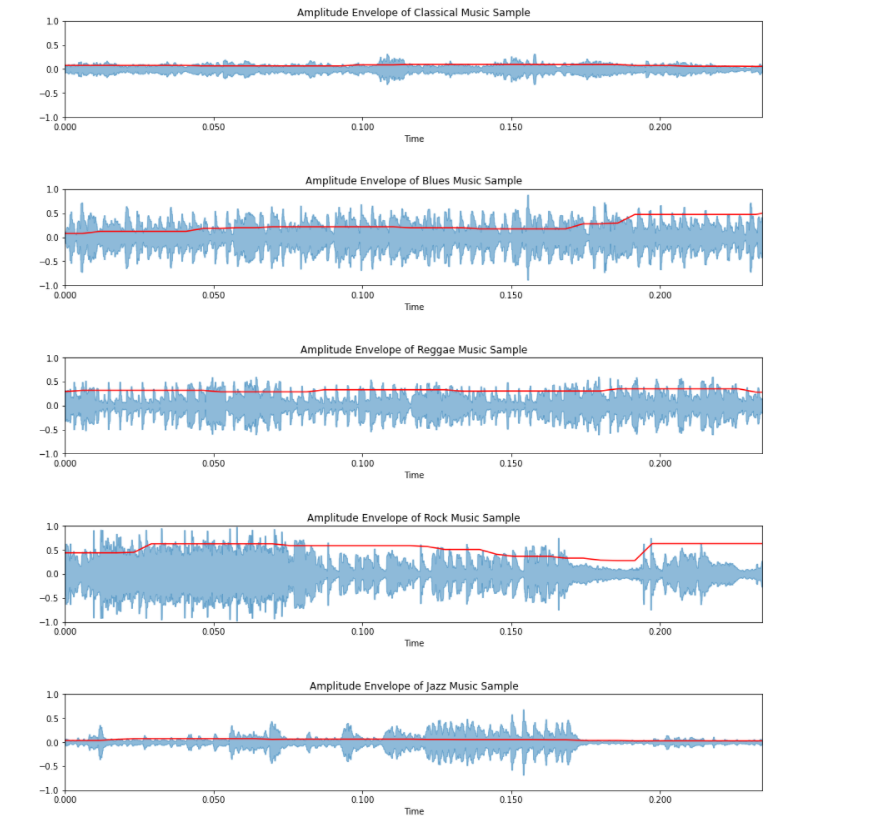
Finally, let’s visualize the amplitude envelops of individual music genres.
Step 6: Visualize the Amplitude Envelope of different music genre tracks
#visualizing Amplitude Envelope
frames = range(0, ae_classical.size)
t = librosa.frames_to_time(frames, hop_length=HOP_LENGTH)
plt.figure(figsize=(15, 17))
plt.subplot(5,1,1)
librosa.display.waveplot(ae_classical, alpha=0.5)
plt.plot(t, ae_classical, color="r")
plt.title("Amplitude Envelope of Classical Music Sample")
plt.ylim(-1,1)
plt.subplot(5,1,2)
librosa.display.waveplot(ae_blues, alpha=0.5)
plt.plot(t, ae_blues, color="r")
plt.title("Amplitude Envelope of Blues Music Sample")
plt.ylim(-1,1)
plt.subplot(5,1,3)
librosa.display.waveplot(ae_reggae, alpha=0.5)
plt.plot(t, ae_reggae, color="r")
plt.title("Amplitude Envelope of Reggae Music Sample")
plt.ylim(-1,1)
plt.subplot(5,1,4)
librosa.display.waveplot(ae_rock, alpha=0.5)
plt.plot(t, ae_rock, color="r")
plt.title("Amplitude Envelope of Rock Music Sample")
plt.ylim(-1,1)
plt.subplot(5,1,5)
librosa.display.waveplot(ae_jazz, alpha=0.5)
plt.plot(t, ae_jazz, color="r")
plt.title("Amplitude Envelope of Jazz Music Sample")
plt.ylim(-1,1)
plt.subplots_adjust(hspace = 0.75)

According to the findings, classical music has the least variability, which means the amplitude envelope is more fluid and has fewer transitions. Furthermore, the amplitude envelope of the audio recording belonging to the jazz music genre is also very consistent (ie. has a longer sustain) throughout time. The audio recording of the rock music genre, on the other hand, had a lot more variation in it.
Applications
To name a few, the amplitude envelope audio function has been widely employed in the following applications:
1. Onset detection: The key objective of onset detection is to identify the start of a musical note or another sound that occurs shortly before the attack.
2. Music Genre classification: The key objective is to analyze the audio signals to determine the genre of music.
3. Studying and surveying the types of sounds
Drawbacks
The amplitude envelope contains a lot of spikes and follows the waveform’s outer contour, making it vulnerable to outliers.
Conclusion
As a result of the aforementioned demonstration, we may conclude that the classical music genre has the least variability. Amplitude envelopes for the classical and even jazz music genres are quite fluid and have fewer transitions. On the other side, we can see that the amplitude envelope for the rock genre, for example, has higher variability in it. However, since it’s a very brief study, we can’t extrapolate these findings entirely, and there may be some differences in observation in some circumstances. Nonetheless, the preceding analysis may provide us with a concise summary, a kind of intuition, concerning distinct types of music genres.
To summarize, the following were the major takeaways from this post for all of us:
- We learned what the Amplitude envelope of audio is.
- We understood the difference between percussive and flat tone amplitude envelopes, as well as their applications in many fields.
- We also used Librosa to visualize the amplitude envelope of different music genre tracks.
- We also learned about the applications and drawbacks of the Amplitude Envelope.
Thank you for taking the time to read this. Please post any questions or concerns you have in the comments section below. Happy learning!
Link to GitHub Repo: Click here!
The media shown in this article is not owned by Analytics Vidhya and is used at the Author’s discretion.


