

In a vector database, we often need to quickly find the most similar results among vast collections of high-dimensional vectors—such as image features, text embeddings, or audio representations. Without an index, the only option is to compare the query vector against every single vector in the dataset. This brute-force search might work when you have a few thousand vectors, but once you’re dealing with tens or hundreds of millions, it becomes unbearably slow and computationally expensive.
That’s where Approximate Nearest Neighbor (ANN) search comes in. Think of it like looking for a specific book in a massive library. Instead of checking every book one by one, you start by browsing the sections most likely to contain it. You might not get the exact same results as a full search, but you’ll get very close—and in a fraction of the time. In short, ANN trades a slight loss in accuracy for a significant boost in speed and scalability.
Among the many ways to implement ANN search, IVF (Inverted File) and HNSW (Hierarchical Navigable Small World) are two of the most widely used. But IVF stands out for its efficiency and adaptability in large-scale vector search. In this article, we’ll walk you through how IVF works and how it compares with HNSW—so you can understand their trade-offs and choose the one that best fits your workload.
What is an IVF Vector Index?
IVF (Inverted File) is one of the most widely used algorithms for ANN. It borrows its core idea from the “inverted index” used in text retrieval systems—only this time, instead of words and documents, we’re dealing with vectors in a high-dimensional space.
Think of it like organizing a massive library. If you dumped every book (vector) into one giant pile, finding what you need would take forever. IVF solves this by first clustering all vectors into groups, or buckets. Each bucket represents a “category” of similar vectors, defined by a centroid—a kind of summary or “label” for everything inside that cluster.
When a query comes in, the search happens in two steps:
1. Find the nearest clusters. The system looks for the few buckets whose centroids are closest to the query vector—just like heading straight to the two or three library sections most likely to have your book.
2. Search within those clusters. Once you’re in the right sections, you only need to look through a small set of books instead of the entire library.
This approach cuts down the amount of computation by orders of magnitude. You still get highly accurate results—but much faster.
How to Build an IVF Vector Index
The process of building an IVF vector index involves three main steps: K-means Clustering, Vector Assignment, and Compression Encoding (Optional). The full process looks like this:
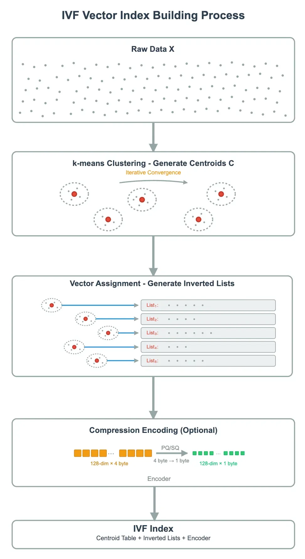
Step 1: K-means Clustering
First, run k-means clustering on the dataset X to divide the high-dimensional vector space into nlist clusters. Each cluster is represented by a centroid, which is stored in the centroid table C. The number of centroids, nlist, is a key hyperparameter that determines how fine-grained the clustering will be.
Here’s how k-means works under the hood:
-
Initialization: Randomly select nlist vectors as the initial centroids.
-
Assignment: For each vector, compute its distance to all centroids and assign it to the nearest one.
-
Update: For each cluster, calculate the average of its vectors and set that as the new centroid.
-
Iteration and convergence: Repeat assignment and update until centroids stop changing significantly or a maximum number of iterations is reached.
Once k-means converges, the resulting nlist centroids form the “index directory” of IVF. They define how the dataset is coarsely partitioned, allowing queries to quickly narrow down the search space later on.
Think back to the library analogy: training centroids is like deciding how to group books by topic:
-
A larger nlist means more sections, each with fewer, more specific books.
-
A smaller nlist means fewer sections, each covering a broader, more mixed range of topics.
Step 2: Vector Assignment
Next, each vector is assigned to the cluster whose centroid it’s closest to, forming inverted lists (List_i). Each inverted list stores the IDs and storage information of all vectors that belong to that cluster.
You can think of this step like shelving the books into their respective sections. When you’re looking for a title later, you only need to check the few sections that are most likely to have it, instead of wandering the whole library.
Step 3: Compression Encoding (Optional)
To save memory and speed up computation, vectors within each cluster can go through compression encoding. There are two common approaches:
-
SQ8 (Scalar Quantization): This method quantizes each dimension of a vector into 8 bits. For a standard
float32vector, each dimension typically takes up 4 bytes. With SQ8, it’s reduced to just 1 byte—achieving a 4:1 compression ratio while keeping the vector’s geometry largely intact. -
PQ (Product Quantization): It splits a high-dimensional vector into several subspaces. For example, a 128-dimensional vector can be divided into 8 sub-vectors of 16 dimensions each. In each subspace, a small codebook (typically with 256 entries) is pre-trained, and each sub-vector is represented by an 8-bit index pointing to its nearest codebook entry. This means the original 128-D
float32vector (which requires 512 bytes) can be represented using only 8 bytes (8 subspaces × 1 byte each), achieving a 64:1 compression ratio.
How to Use the IVF Vector Index for Search
Once the centroid table, inverted lists, and the compression encoder and codebooks (optional) are built, the IVF index can be used to accelerate similarity search. The process typically has three main steps, as shown below:
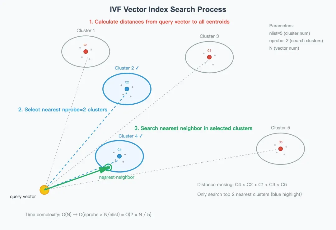
Step 1: Calculate distances from the query vector to all centroids
When a query vector q arrives, the system first determines which clusters it is most likely to belong to. Then, it computes the distance between q and every centroid in the centroid table C—usually using Euclidean distance or inner product as the similarity metric. The centroids are then sorted by their distance to the query vector, producing an ordered list from nearest to farthest.
For example, as shown in the illustration, the order is: C4 < C2 < C1 < C3 < C5.
Step 2: Select the nearest nprobe clusters
To avoid scanning the entire dataset, IVF only searches within the top nprobe clusters that are closest to the query vector.
The parameter nprobe defines the search scope and directly affects the balance between speed and recall:
-
A smaller nprobe leads to faster queries but may reduce recall.
-
A larger nprobe improves recall but increases latency.
In real-world systems, nprobe can be dynamically tuned based on the latency budget or accuracy requirements.
In the example above, if nprobe = 2, the system will only search within Cluster 2 and Cluster 4—the two nearest clusters.
Step 3: Search the nearest neighbor in the selected clusters
Once the candidate clusters are selected, the system compares the query vector q with the vectors stored inside them.
There are two main modes of comparison:
-
Exact Comparison (IVF_FLAT): The system retrieves the original vectors from the selected clusters and computes their distances to q directly, returning the most accurate results.
-
Approximate Comparison (IVF_PQ / IVF_SQ8): When PQ or SQ8 compression is used, the system employs a lookup table method to accelerate distance computation. Before the search begins, it precomputes the distances between the query vector and each codebook entry. Then, for each vector, it can simply “look up and sum” these precomputed distances to estimate similarity.
Finally, the candidate results from all searched clusters are merged and re-ranked, producing the Top-k most similar vectors as the final output.
IVF In-Practice
Once you understand how IVF vector indexes are built and searched, the next step is to apply them for real-world workloads. In practice, you’ll often need to balance performance, accuracy, and memory usage. Below are some practical guidelines drawn from engineering experience.
How to Choose the Right nlist
As mentioned earlier, the parameter nlist determines the number of clusters into which the dataset is divided when building an IVF index.
-
Larger nlist: Creates finer-grained clusters, meaning each cluster contains fewer vectors. This reduces the number of vectors scanned during search and generally results in faster queries. But building the index takes longer, and the centroid table consumes more memory.
-
Smaller nlist: Speeds up index construction and reduces memory usage, but each cluster becomes more “crowded.” Each query must scan more vectors within a cluster, which can lead to performance bottlenecks.
Based on these trade-offs, here’s a practical rule of thumb:
For datasets at the million scale, a good starting point is nlist ≈ √n (n is the number of vectors in the data shard being indexed).
For example, if you have 1 million vectors, try nlist = 1,000. For larger datasets—tens or hundreds of millions—most vector databases shard the data so that each shard contains around one million vectors, keeping this rule practical.
Because nlist is fixed at index creation, changing it later means rebuilding the entire index. So it’s best to experiment early. Test several values—ideally in powers of two (e.g., 1024, 2048)—to find the sweet spot that balances speed, accuracy, and memory for your workload.
How to Tune nprobe
The parameter nprobe controls the number of clusters searched during query time. It directly affects the trade-off between recall and latency.
-
Larger nprobe: Covers more clusters, leading to higher recall but also higher latency. The delay generally increases linearly with the number of clusters searched.
-
Smaller nprobe: Searches fewer clusters, resulting in lower latency and faster queries. However, it may miss some true nearest neighbors, slightly lowering recall and result accuracy.
If your application is not extremely sensitive to latency, it’s a good idea to experiment with nprobe dynamically—for example, testing values from 1 to 16 to observe how recall and latency change. The goal is to find the sweet spot where recall is acceptable and latency remains within your target range.
Since nprobe is a runtime search parameter, it can be adjusted on the fly without requiring the index to be rebuilt. This enables fast, low-cost, and highly flexible tuning across different workloads or query scenarios.
Common Variants of the IVF Index
When building an IVF index, you’ll need to decide whether to use compression encoding for the vectors in each cluster—and if so, which method to use.
This results in three common IVF index variants:
| IVF Variant | Key Features | Use Cases |
|---|---|---|
| IVF_FLAT | Stores raw vectors within each cluster without compression. Offers the highest accuracy, but also consumes the most memory. | Ideal for medium-scale datasets (up to hundreds of millions of vectors) where high recall (95%+) is required. |
| IVF_PQ | Applies Product Quantization (PQ) to compress vectors within clusters. By adjusting the compression ratio, memory usage can be significantly reduced. | Suitable for large-scale vector search (hundreds of millions or more) where some accuracy loss is acceptable. With a 64:1 compression ratio, recall is typically around 70%, but can reach 90% or higher by lowering the compression ratio. |
| IVF_SQ8 | Uses Scalar Quantization (SQ8) to quantize vectors. Memory usage sits between IVF_FLAT and IVF_PQ. | Ideal for large-scale vector search where you need to maintain relatively high recall (90%+) while improving efficiency. |
IVF vs HNSW: Pick What Fits
Besides IVF, HNSW (Hierarchical Navigable Small World) is another widely used in-memory vector index. The table below highlights the key differences between the two.
| IVF | HNSW | |
|---|---|---|
| Algorithm Concept | Clustering and bucketing | Multi-layer graph navigation |
| Memory Usage | Relatively low | Relatively high |
| Index Build Speed | Fast (only requires clustering) | Slow (needs multi-layer graph construction) |
| Query Speed (No Filtering) | Fast, depends on nprobe | Extremely fast, but with logarithmic complexity |
| Query Speed (With Filtering) | Stable — performs coarse filtering at the centroid level to narrow down candidates | Unstable — especially when the filtering ratio is high (90%+), the graph becomes fragmented and may degrade to near full-graph traversal, even slower than brute-force search |
| Recall Rate | Depends on whether compression is used; without quantization, recall can reach 95%+ | Usually higher, around 98%+ |
| Key Parameters | nlist, nprobe | m, ef_construction, ef_search |
| Use Cases | When memory is limited, but high query performance and recall are required; well-suited for searches with filtering conditions | When memory is sufficient and the goal is extremely high recall and query performance, but filtering is not needed, or the filtering ratio is low |
In real-world applications, it’s very common to include filtering conditions—for example, “only search vectors from a specific user” or “limit results to a certain time range.” Due to differences in their underlying algorithms, IVF generally handles filtered searches more efficiently than HNSW.
The strength of IVF lies in its two-level filtering process. It can first perform a coarse-grained filter at the centroid (cluster) level to quickly narrow down the candidate set, and then conduct fine-grained distance calculations within the selected clusters. This maintains stable and predictable performance, even when a large portion of the data is filtered out.
In contrast, HNSW is based on graph traversal. Because of its structure, it cannot directly leverage filtering conditions during traversal. When the filtering ratio is low, this doesn’t cause major issues. However, when the filtering ratio is high (e.g., more than 90% of data is filtered out), the remaining graph often becomes fragmented, forming many “isolated nodes.” In such cases, the search may degrade into a near full-graph traversal—sometimes even worse than a brute-force search.
In practice, IVF indexes are already powering many high-impact use cases across different domains:
-
E-commerce search: A user can upload a product image and instantly find visually similar items from millions of listings.
-
Patent retrieval: Given a short description, the system can locate the most semantically related patents from a massive database—far more efficient than traditional keyword search.
-
RAG knowledge bases: IVF helps retrieve the most relevant context from millions of tenant documents, ensuring AI models generate more accurate and grounded responses.
Conclusion
To choose the right index, it all comes down to your specific use case. If you’re working with large-scale datasets or need to support filtered searches, IVF can be the better fit. Compared with graph-based indexes like HNSW, IVF delivers faster index builds, lower memory usage, and a strong balance between speed and accuracy.
Milvus, the most popular open-source vector database, provides full support for the entire IVF family, including IVF_FLAT, IVF_PQ, and IVF_SQ8. You can easily experiment with these index types and find the setup that best fits your performance and memory needs. For a complete list of indexes Milvus supports, check out this Milvus Index doc page.
If you’re building image search, recommendation systems, or RAG knowledge bases, give IVF indexing in Milvus a try—and see how efficient, large-scale vector search feels in action.
… [Trackback]
[…] Find More on on that Topic: geeksforgeeks.org/understanding-ivf-vector-index-how-it-works-and-when-to-choose-it-over-hnsw/ […]
… [Trackback]
[…] Here you can find 82466 additional Information on that Topic: geeksforgeeks.org/understanding-ivf-vector-index-how-it-works-and-when-to-choose-it-over-hnsw/ […]