

In the beginning, learning Machine Learning (ML) can be intimidating. Terms like “Gradient Descent”, “Latent Dirichlet Allocation” or “Convolutional Layer” can scare lots of people. But there are friendly ways of getting into the discipline, and I think starting with this guide to decision trees is a wise decision.
Decision Trees (DTs) are probably one of the most useful supervised learning algorithms out there. As opposed to unsupervised learning (where there is no output variable to guide the learning process and data is explored by algorithms to find patterns), in supervised learning your existing data is already labeled and you know which behavior you want to predict in the new data you obtain. This is the type of algorithms that autonomous cars use to recognize pedestrians and objects, or organizations exploit to estimate customers lifetime value and their churn rates.
In a way, supervised learning is like learning with a teacher, and then apply that knowledge to new data.
The Guide to Decision Trees
DTs are ML algorithms that progressively divide data sets into smaller data groups based on a descriptive feature, until they reach sets that are small enough to be described by some label. They require that you have data that is labeled (tagged with one or more labels, like the plant name in pictures of plants), so they try to label new data based on that knowledge.
[Related article: Why Do Tree Ensembles Work?]
DTs algorithms are perfect to solve classification (where machines sort data into classes, like whether an email is spam or not) and regression (where machines predict values, like a property price) problems. Regression Trees are used when the dependent variable is continuous or quantitative (e.g. if we want to estimate the probability that a customer will default on a loan), and Classification Trees are used when the dependent variable is categorical or qualitative (e.g. if we want to estimate the blood type of a person).
The importance of DTs relies on the fact that they have lots of applications in the real world. Being one of the most used algorithms in ML, they are applied to different functionalities in several industries:
-DTs are being used in the healthcare industry to improve the screening of positive cases in the early detection of cognitive impairment, and also to identify the main risk factors of developing some type of dementia in the future.
-Sophia, the robot that was made a citizen of Saudi Arabia, uses DTs algorithms to chat with humans. In fact, chatbots that use these algorithms are already bringing benefits in industries like health insurance by gathering data from customers through the application of innovative surveys and friendly chats. Google recently acquired Onward, a company that uses DTs to develop chatbots that are exceptionally functional in delivering world-class customer care, and Amazon is investing in the same direction to guide customers quickly to a path of resolution.
-It is possible to predict the most likely causes of forest disturbances, like wildfire, logging of tree plantations, large or small scale agriculture, and urbanization by training DTs to recognize different causes of forest loss from satellite imagery. DTs and satellite imagery are also used in agriculture to classify different crop types and identify their phenological stages.
-DTs are great tools to perform sentiment analysis of texts, and identify the emotions behind them. Sentiment analysis is a powerful technique that can help organizations to learn about customers choices and their decision drivers.
-In environmental sciences, DTs can help to determine the best strategy for dealing with invasive species, ranging from eradication to containment, and mitigation of spread.
-DTs are also used to improve financial fraud detection. The MIT showed that it could significantly improve the performance of alternative ML models by using DTs that were trained with several sources of raw data to find patterns of transactions and credit cards that match cases of fraud.
DTs are extremely popular for a variety of reasons, being their interpretability probably their most important advantage. They can be trained very fast and are easy to understand, which opens their possibilities to frontiers far beyond scientific walls. Nowadays, DTs are very popular in business environments and their usage is also expanding to civil areas, where some applications are raising big concerns.
The firm Sesame Credit (a company affiliated with Alibaba) uses DTs and other algorithms to engine a system of social evaluation, taking into consideration various factors such as the punctuality with which bills are paid and other online activities. The benefits of a good “Sesame score” in China range from a higher visibility on dating sites to skipping the waiting line if you need to see a doctor. Actually, after the Chinese government announced it will apply its so-called social credit system to flights and trains and stop people who have committed misdeeds from taking such transport for up to a year, there is a concern that the system will end up creating a massive “ML-backed Big Brother”.
The Basics
In the movie Bandersnatch (a stand-alone Black Mirror episode from Netflix), the viewer can interactively choose different narrative paths and reach different storylines and endings. There is a complex set of decisions hidden behind the movie storytelling that lets the audience move in a kind of Choose Your Own Adventure mode, for which Netflix had to work out a way of loading multiple versions of each scene while presenting it in a simple way. In practice, what Netflix producers did was to segment the movie and set different branch points for the viewer to move through, and come up with different results. In other words, this is just like building a DT.
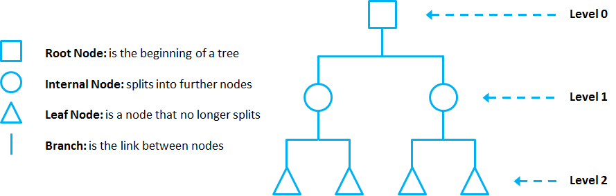
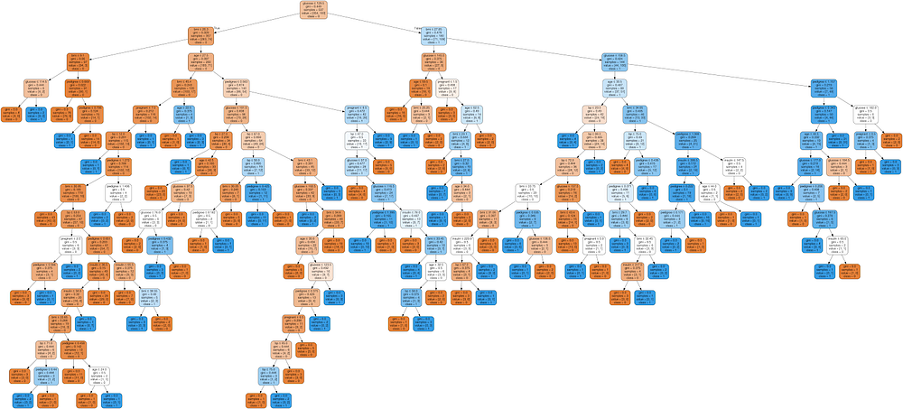
DTs are composed of nodes, branches, and leaves. Each node represents an attribute (or feature), each branch represents a rule (or decision), and each leaf represents an outcome. The depth of a Tree is defined by the number of levels, not including the root node.
DTs apply a top-down approach to data, so that given a data set, they try to group and label observations that are similar between them, and look for the best rules that split the observations that are dissimilar between them until they reach a certain degree of similarity.
They use a layered splitting process, where at each layer they try to split the data into two or more groups, so that data that fall into the same group are most similar to each other (homogeneity), and groups are as different as possible from each other (heterogeneity).
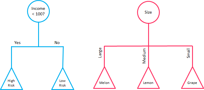
The splitting can be binary (which splits each node into at most two sub-groups, and tries to find the optimal partitioning), or multiway (which splits each node into multiple sub-groups, using as many partitions as existing distinct values). In practice, it is usual to see DTs with binary splits, but it’s important to know that multiway splitting has some advantages. Multiway splits exhaust all information in a nominal attribute, which means that an attribute rarely appears more than once in any path from the root to the leaf, which make DTs easier to comprehend. In fact, it could happen that the best way to split data might be to find a set of intervals for a given feature, and then split that data up into several groups based on those intervals.
In bidimensional terms (using only 2 variables), DTs partition the data universe into a set of rectangles, and fit a model in each one of those rectangles. They are simple yet powerful, and a great tool for data scientists.
Each node in the DT acts as a test case for some condition, and each branch descending from that node corresponds to one of the possible answers to that test case.
Prune that Tree
As the number of splits in DTs increase, their complexity rises. In general, simpler DTs are preferred over super complex ones, since they are easier to understand and they are less likely to fall into overfitting.
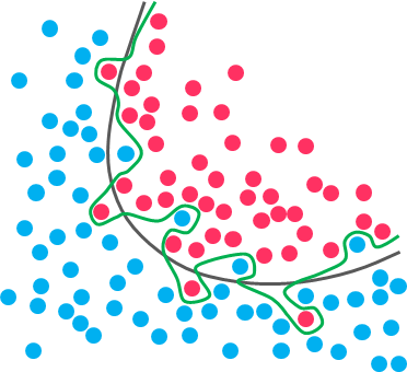
Overfitting refers to a model that learns the training data (the data it uses to learn) so well that it has problems to generalize to new (unseen) data.
In other words, the model learns the detail and noise (irrelevant information or randomness in a dataset) in the training data to the extent that it negatively impacts the performance of the model on new data. This means that the noise or random fluctuations in the training data is picked up and learned as concepts by the model.
[20 Free ODSC Resources to Learn Machine Learning]
Under this condition, your model works perfectly well with the data you provide upfront, but when you expose that same model to new data, it breaks down. It’s unable to repeat its highly detailed performance.
So, how do you avoid overfitting in DTs? You need to exclude branches that fit data too specifically. You want a DT that can generalize and work well on new data, even though this may imply losing precision on the training data. It’s always better to avoid a DT model that learns and repeats specific details like a parrot, and try to develop one that has the power and flexibility to have a decent performance on new data you provide to it.
Pruning is a technique used to deal with overfitting, that reduces the size of DTs by removing sections of the Tree that provide little predictive or classification power.
The goal of this procedure is to reduce complexity and gain better accuracy by reducing the effects of overfitting and removing sections of the DT that may be based on noisy or erroneous data. There are two different strategies to perform pruning on DTs:
- Pre-prune: When you stop growing DT branches when information becomes unreliable.
- Post-prune: When you take a fully grown DT and then remove leaf nodes only if it results in a better model performance. This way, you stop removing nodes when no further improvements can be made.
In summary, a big DT that correctly classifies or predicts every example of the training data might not be as good as a smaller one that does not fit all the training data perfectly.