This article was published as a part of the Data Science Blogathon.
Introduction
Suppose you are at a company for a job interview, and your friend has gone in for the interview before you. You estimate your chances of selection to be low, but when you hear from your friend that the interview was pretty easy and he/she feels that they have a good chance at being selected, wouldn’t you re-estimate your chances as well? Well, that’s the essence of Bayes’ theorem.
The Bayes’ theorem is perhaps the most important in the context of probabilities. In simple terms, Bayes’ theorem helps us update our prior beliefs based on some new evidence. This is probably the gist of the Bayes theorem. I’m sure there are quite a few question marks on your mind but don’t worry, I have got you covered :).
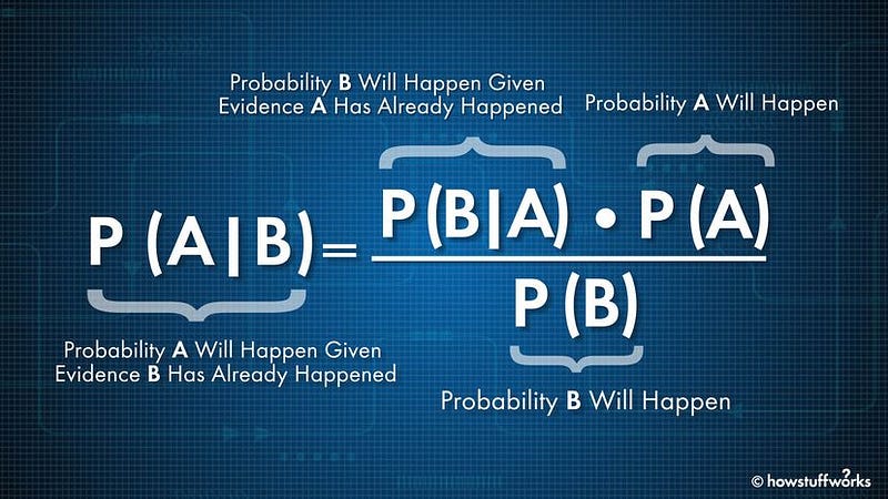
Before getting into Bayes’ theorem, we’ll have to brush up on the concept of conditional probability. The traditional probability can be explained as the ratio of the number of events favorable to the total number of events. Utilizing this, one can derive the conditional probability formula, which is event A’s probability given that event B has occurred. Therefore, the above formula will be modified to,


Illustration using Marbles
Bag 1– 2 white, 3 black marbles
Bag 2– 4 white, 2 black marbles
Now, if I asked you to calculate the probability of getting a white marble from bag 1, you would easily be able to calculate that right? (2/5 = 40%) On the flip side, if I said that white marble is drawn, determine the probability that it came from bag 2. How would you calculate that?
Enter ‘Reverend Thomas Bayes’. He found that if you can estimate the values of P(A), P(B), and the conditional probability P(B|A), you can compute the conditional probability P(A|B). That’s why this theorem is also called the ‘probability of causes’.
Event A — Getting a white marble
Event E1 — Choosing bag 1
Event E2 — Choosing bag 2
P (choosing bag 1) = P(E1) = P(choosing bag 2) = P(E2) = 1/2
P(white marble, given that it’s from bag 1) = P(A|E1)= 2/5
P(white marble given that it’s from bag 2) = P(A|E2) = 4/6
To find, Probability of drawing a marble from bag 2, given that it’s white marble. With the help of Bayes’ theorem, we can find the P(E2|A).

After plugging in the values in the above formula, you should get your answer.
Illustration using Football
To understand it better, let’s take an out-of-the-textbook example.
Mohamed Salah is a world-class footballer who plays as a Liverpool FC forward. He is predominantly a left-footed player. Hence he takes a higher number of shots from his left foot.
Let us find out the chances that he took the shot from his right foot, given that the shot was a goal.
Note: xG (expected goal) is a measure of shot quality; what are the chances of scoring a goal from that position based on records.
Let the events be as follows,
A — scoring a goal
E1 — the shot was taken from the right foot
E2 — the shot was taken from the left foot
As shown below, Mo Salah had a total of 139 shots in the 2021–22 season. Therefore,
P(shot was taken from right) = P(E1) = 15/139 = 0.1079
P(shot was taken from left) = P(E2) = 117/139 = 0.8417
Now for the conditional probabilities, which will be equal to the xG/shot for that particular foot.
P(scoring a goal given shot was taken from the right foot) = P(A|E1) = 0.27
P(scoring a goal given shot was taken from the left foot) = P(A|E2) = 0.16

Now all that remains is to put the values in the formula mentioned in the first example, and boom, you have your answer.

So the chances that Mo Salah took the shot from his right foot, given that the shot was a goal, is 0.1779 ~ 18%. Therefore, there’s an 18% chance that the shot was taken from the right, given that it was a goal. Similarly, can you determine the probability that Mo Salah took the shot from his left foot, given that the outcome was a goal? Let me know the answer in the comments.
Bayes theorem in ML
After understanding Bayes’ theorem, let’s quickly try to understand its use in machine learning. The naive Bayes theorem is one of the fastest machine learning algorithms, and the best part is that it’s straightforward to interpret.
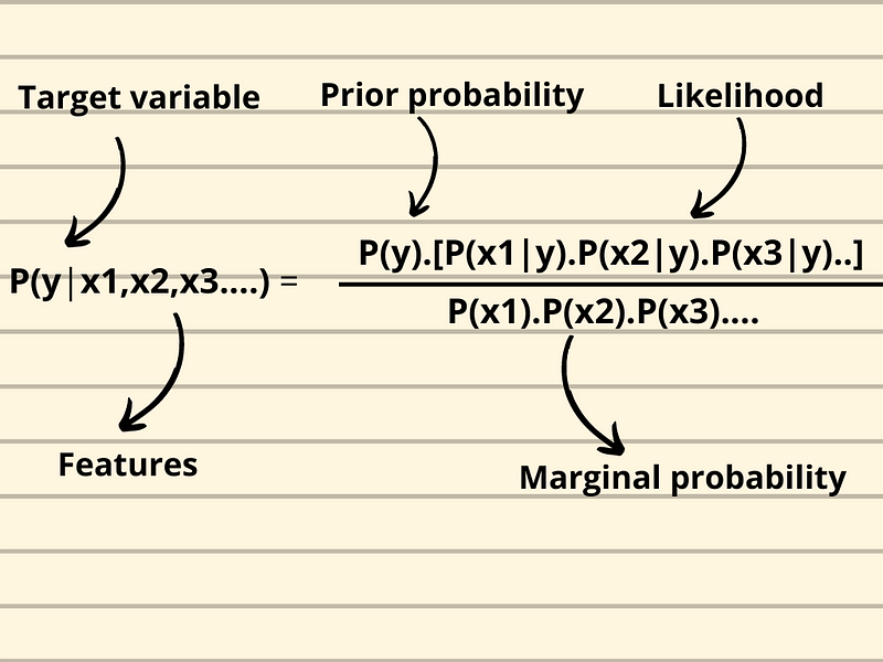
The model is used for classification, be it binary or multi-class classification. The end goal is to get the maximum posterior probability of a class, and that will be assigned as the predicted class.

As illustrated in the graphic above, one can calculate the posterior probability of each class given the features and select the maximum posterior probability, also called Maximum A Posteriori (MAP). The marginal probability is constant for each class and is only used for normalizing the result.
The Naive Bayes classifier is fast and can provide real-time results. It is widely used in text classification for sentiment analysis. There are different types of Naive Bayes models, depending on the data type.
Gaussian
- normal distribution
- continuous values
Multinomial:
- multinomial distribution
- multinomial categorical variables
Bernoulli:
- binomial distribution
- binary categorical variables
The Naive Bayes model assumes that the features are independent, meaning the data has no multicollinearity, which is not the case in real-world problems. Despite this, the model has worked well in various classification problems such as spam filtering.
Win Predictor Using Naive Bayes Model
Let’s implement the Naive Bayes model in python to better understand the model. We start by importing the data and the required libraries. The data is scraped from fotmob.com; you can check out the tutorial here.
The dataset did not have the results column. Hence I added that.
#Home — 1
#Away — 2
#Draw — 0
results = []
result = 0
for i in range(len(df)):
  if df.home_team_score[i] > df.away_team_score[i]:
     result = 1
     results.append(result)
  elif df.home_team_score[i] < df.away_team_score[i]:
     result = 2
     results.append(result)
  else:
     result = 0
     results.append(result)
df['result'] = results
Next, I replaced the team names with numbers.
df.replace({‘ATK Mohun Bagan FC’:1, ‘Bengaluru FC’:2,
            ‘SC East Bengal’:3,‘Mumbai City FC’:4, ‘Hyderabad FC’:5,
            ‘Odisha FC’:6,‘Northeast United FC’:7, ‘FC Goa’:8,
‘Jamshedpur’:9,'Chennaiyin FC’:10,‘Kerala Blasters FC’:11},inplace=True)
Training the model and predicting the results.
X = df.drop(['result'],axis=1)
y = df['result']
X_train, X_test, y_train, y_test = train_test_split(X, y, test_size=0.2, random_state=0)
gnb = GaussianNB()
y_pred = gnb.fit(X_train, y_train).predict(X_test)
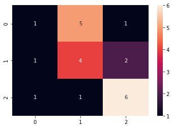
cf = confusion_matrix(y_test,y_pred)
sns.heatmap(cf, annot=True)

The model had a decent output considering there were just 110 data points in the data set. The accuracy can be increased through feature engineering and training it more data points.
Conclusion
The Bayes theorem is one of the simplest but beneficial probability theorems. It lays the foundation for various machine learning models, such as the Naive Bayes model. Although keep in mind the Naive Bayes model assumes no correlation between the features.
The science of probability is extremely captivating and especially for data enthusiasts. Predicting outcomes is the day-to-day job of a data scientist; therefore, understanding the machine learning models is crucial to optimize results.
To summarise the article:
- Bayes theorem is a scientific approach to updating prior beliefs given new evidence. That is, if the probability of events A, B, and (B given A) is available, then you can compute P(A given B).
- It is used in several sectors like finance, sports, and health to estimate the odds.
- It lays the foundation for machine learning models such as the Naive Bayes theorem
- The Naive Bayes model is mostly employed in spam filtering, sentiment analysis, and recommendation systems.
I hope this article helped you understand the theorem and its usage in machine learning. Let me know in the comments if you have any doubts regarding the theorem.
The media shown in this article is not owned by Analytics Vidhya and is used at the Author’s discretion.


