What you will learn in this Article
In this article, we will see every single details that you need to know for sentiment data analysis using the LSTM network using the torchtext library. We will see, how to use spacy tokenizer in torchtext data class and the use of tabular and bucket iterator. We will use the embedding matrix with or without pre-trained Glove embedding as an input and we will also see how to process text data of different lengths in a batch with pack_padded_sequence. And you can use these techniques in your problem
What are Field and LabelField?
In sentiment data, we have text data and labels (sentiments). The torchtext came up with its text processing data types in NLP. The text data is used with data-type: Field and the data type for the class are LabelField. In the older version PyTorch, you can import these data-types from torchtext.data but in the new version, you will find it in torchtext.legacy.data. You can find detailed information for Field here.
Some important arguments of the data types, that you will use are ‘tokenize’, ‘use_vocab’, ‘batch_first’, ‘include_lengths’, ‘sequential’, and ‘lower’. Let’s first understand the argument tokenize. In simple words, tokenization is a process to split your sentence into words or more basic words. You can use tokenize in many ways either defining your function of a tokenizer, or you can define a function in torch with get_tokenizer, or you can use an inbuilt tokenizer of Field. First, we will install spacy then we will see the tokenizer function.
pip install spacy
python -m spacy download en_core_web_sm
# Build tokenizer
def tokenizer(text):
    return [token.text for token in spacy_en.tokenizer(text)]
You can also define using torch get_tokenizer as well (another way to define) :
from torchtext.data.utils import get_tokenizer
tokenizer = get_tokenizer('spacy', language='en_core_web_sm')
Let’s see the output of any of the tokenizer we defined above. Both are the same.
print(tokenizer("I can't run whole day"))
Output:
['I', 'ca', "n't", 'run', 'whole', 'day']
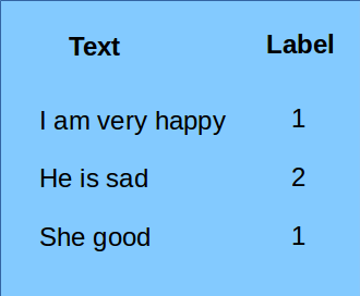
After defining the tokenizer, you can pass it into your Filed. Filed is data-type for your input text. For the article purpose let’s define some sample data in a CSV file.
TEXT = data.Field(tokenize=tokenizer, use_vocab=True, lower=True, batch_first=True, include_lengths=True)
LABEL = data.LabelField(dtype=torch.long, batch_first=True, sequential=False)
fields = [('text', TEXT), ('label', LABEL)]
In the above data-set and the code: Text input is sequential data and sequential argument is True by default so no need to pass in the first line of code and we pass it in the label field. The include_lengths argument will return the length of each sentence in a batch, we will see this in BucketIterator section of this article in more detail. We can also use tokenizer within the Field without using any tokenizer function we did above (we are not using any of the tokenizer functions we defined above)-
TEXT = data.Field(use_vocab=True, lower=True, tokenize='spacy', tokenizer_language='en_core_web_sm', batch_first=True, include_lengths=True)
TabularDataset for the Project
In torchtext we have TabularDataset and it is a very useful class for NLP purposes, which reads the data in any format CSV, TSV, or JSON. The field argument will be passed in this class. We have defined the class and iterate the class to see our data below.
training_data = data.TabularDataset(
    path='sample.csv',
    format='csv',
    fields=fields,
    skip_header=True,
)
for example in training_data.examples:
    print(example.text, example.label)
Output:
['she', 'good'] 1
['he', 'is', 'sad'] 2
['i', 'am', 'very', 'happy'] 1
We will do the same thing we do always, splitting data into trains and test data as we do with train_test_split of Sklearn. Here TabularDataset has a split function itself, and we will use that function to split our data with a random state:
train_data, val_data = training_data.split(split_ratio=0.7, random_state=random.seed(SEED))
Glove Embedding for Sentiment Analysis LSTM TorchText
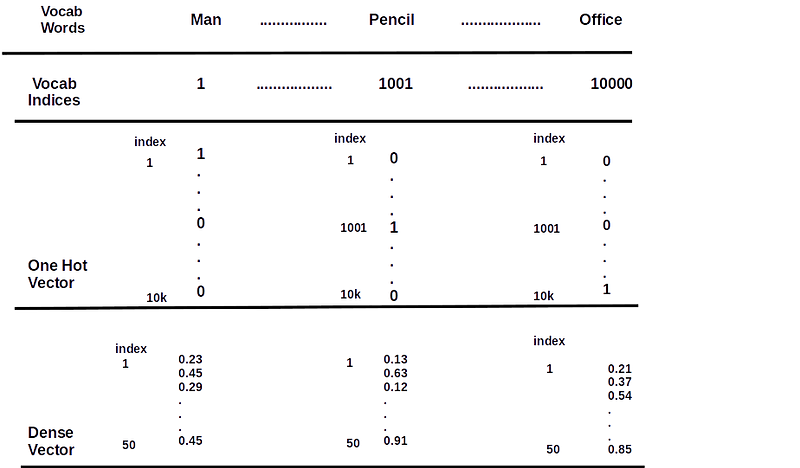
Up to this point, we have read our data and converted it into TabularDataset. Now we will see, how to use embedding in this data. I am giving basic informative notes on embedding, which will be helpful for you if you are not aware. Neural Net only deals with numbers. Embedding converts words into integers and there is a vector corresponding to each integer. Refer to the below image, suppose we have 10k words in our dictionary and you have assigned each word a value between1 to 10k.
Create a zero vector of dimension 10k, Now suppose if you want to represent the word “man”, because its value is 1 in the dictionary(refer to the image below), so in the vector put 1 in the first index and keep others to zero. Such types of vectors are one-hot encode vectors and the problem with these vectors is their dimension. If we have 2B words in our dictionary, we have to make a 2B dimension vector.
To overcome such a problem we generate a dense vector and Glove is one such approach that has a dense vector for a word. Here we will download and use pre-trained Glove Embedding in our problem. You can download the Glove vector using the torch and all the dimensional details can be found at this link.

Figure 2: vectors representation of words
vectors = Vectors(name='glove.6B.50d.txt')
TEXT.build_vocab(train_data, vectors=vectors, max_size=10000, min_freq=1)
LABEL.build_vocab(train_data)
In the above code, we initialized the vector and build our training data vocabulary with this vector. I mean, we get a vector for all known tokens from the data set (word/ token). We can restrict the size of vocabulary also. If you do not have the Glove text file, use the following code to download the vector. The cache argument will help you to store the downloaded file for future use. I mean, no need to download the same file again and again.
cache = '.vector_cache'
if not os.path.exists(cache):
    os.mkdir(cache)
vectors = Glove(name='840B', dim=50, cache=cache)
When you have built the vocabulary, you can check out the dictionary. Here I have small data so I can print whole tokens here for demonstration purposes.
print(list(TEXT.vocab.stoi.items()))
output:
[('', 0), ('', 1), ('am', 2), ('good', 3), ('happy', 4), ('he', 5), ('i', 6), ('is', 7), ('sad', 8), ('she', 9), ('very', 10)]
If you have noticed, we have two extra tokens UNK and PAD and the corresponding indices of these two are 0 and 1. If you want to see the vector corresponding to token=’good’, you can do this by the code below.
print(TEXT.vocab.vectors[TEXT.vocab.stoi['good']])
Here TEXT.vocab.vectors contains 50 dimensional vectors for 11 different tokens. TEXT.vocab.stoi converts string to integer(index). The vectors for UNK and PAD are always zero vectors. I am not printing the values as it will take more space here, but you can play around with it. Now I am getting the device type I have because it is going to be used in Bucket-Iterator.
device = torch.device('cuda' if torch.cuda.is_available() else 'cpu')
BucketIterator for Sentiment Analysis LSTM TorchText
Before the code part of BucketIterator, let’s understand the need for it. This iterator rearranges our data so that similar lengths of sequences fall in one batch with descending order to sequence length (seq_len=Number of tokens in a sentence). If we have the text of length=[4,6,8,5] and we want to split this data into two batches the BucketIterator will split it into [8,6] and [5,4].

Arranging data in descending order is required for efficient calculations. Should we replace the question mark with PAD tokens? You will get the answer in this article. BucketIterator helps to keep a similar length of sentences in one batch. This will reduce the padding tokens overhead for computational points of view, first see how to code the BucketIterator:
BTACH_SZIE = 2
train_itr, val_itr = BucketIterator.splits(
    (train_data, val_data),
    batch_size=BATCH_SIZE,
    sort_key=lambda x:len(x.text),
    device=device,
    shuffle=True,
    sort_within_batch=True,
    sort=False
)
I hope every argument is self-explanatory here, we passed the batch size of 2. Choose batch size wisely as it is a crucial hyper-parameter and its value also depends on how much data you can process in your GPU/CPU memory. We did not sort the entire data-set but we did sort the data samples within a batch(sort_within_batch=True). See how our batches look:
for batch_no, batch in enumerate(train_itr):
    text, batch_len = batch.text
    print(text, batch_len)
    print(batch.label)
output:
(tensor([[ 6,  2, 10,  4],
        [ 5,  7,  8,  1]]), tensor([4, 3]))
 tensor([0, 1])
Each batch contains the token ids and labels, here we got the length of each sentence in a batch as well because we passed include_length as true in the TEXT Field. If you have more sentences of different lengths, you will see BucketIterator arrange the data very nicely.
Basics of LSTM Model
Long short-term memory (LSTM) is a family member of RNN. RNN learns the sequential relationship and this is the reason RNN works well in NLP because the next token has some information from the previous tokens. LSTM can learn longer sequences compare to RNN or GRU. Example: “I am not going to say sorry, and this is not my fault.”
Here the same person who does not want to say sorry is also confident of not being guilty. To understand such logic the network has to be capable of learning the relationship between the first word to the last word of a sentence if necessary. For longer sentences, the network has to understand the relevant relationship between all words and the order of the sequence (which token is coming next in the sentence).
The LSTM plays a very good role here and remembers longer dependency in the sequence due to its capability of remembering relevant information and forgetting irreverent information in a sequence. You can explore this article for more details, you will get all the RNN basics.
Input Shape and Hidden
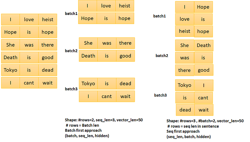
The input can be given in two ways: 1. (Sequence First: Sequence Length, Batch Size, Input Dimension) 2. (Batch First: Batch Size, Sequence Length, Input Dimension). We will use the second format of the input here. We already have defined the batch size in the BucketIterator, the sequence_length is the number of tokens in a batch and the input dimension is the Glove vector dimension which is 50 in our case.
The hidden shape is (No of Direction * Number of Layers, Batch Size, Hidden Size). Sentiment text information can be extracted using Bi-directional LSTM so the number of directions is 2, we will use 2 number of LSTM layers so its value is 2 in our case. The batch size we already discussed and hidden size you can choose suitable value 8, 16, 32, 64, etc.

Model
class SentimentClassifier(nn.Module):
    def __init__(self, vocab_size, embed_dim,
                 hidden, n_label, n_layers):
        super(SentimentClassifier, self).__init__()
        self.hidden = hidden
        self.n_layers = n_layers
        self.embed = nn.Embedding(vocab_size, embed_dim)
        self.lstm = nn.LSTM(embed_dim, hidden,
                            num_layers=n_layers,
                            bidirectional=True,
                            batch_first=True)#dropout=0.2
        self.fc = nn.Linear(hidden * 2, n_label)
    def forward(self, input, actual_batch_len):
        embed_out = self.embed(input)
        hidden = torch.zeros(self.n_layers * 2 ,
                             input.shape[0], self.hidden)
        cell = torch.zeros( self.n_layers * 2,
                            input.shape[0], self.hidden)
        pack_out = nn.utils.rnn.pack_padded_sequence(
            embed_out, actual_batch_len,batch_first=True).to(device)
        out_lstm, (hidden, cell) = self.lstm(pack_out,
                                             (hidden, cell))#dropout
        hidden = torch.cat((hidden[-2,:,:], hidden[-1,:,:]),dim=1)
        out = self.fc(hidden)
        return out
VOCAB_SIZE = len(TEXT.vocab)
EMBEDDING_DIM = TEXT.vocab.vectors.shape[1]
HIDDEN= 64
NUM_LABEL = 4 # number of classes
NUM_LAYERS = 2
model = SentimentClassifier(VOCAB_SIZE, EMBEDDING_DIM, HIDDEN, NUM_LABEL, NUM_LAYERS)
This is our model, do not worry we will break this code step by step. VOCAB_SIZE: Total tokens in data set, EMBEDDING_DIM: Glove vector dimension (50 here), HIDDEN we took 64, NUM_LABEL is our number of classes and NUM_LAYERS is 2: 2 stacked LSTM layer. First, we defined the embedding layer which is a mapping of the vocabulary size to a dense vector, this is the reason, we have mapped total vocab size to the vector dimension. See an example for torch embedding where we have only 2 tokens in the vocab and we want it to transform into a 4-dimensional vector:
emb = nn.Embedding(2,4)# size of vocab = 2, vector len = 4
print(emb.weight)
output:
tensor([[ 0.2626, -0.7775, -0.7230,  0.6391],
        [-0.7772,  0.4914, -0.9622,  1.2316]], requires_grad=True)
In the above code, the first and second output list is a 4-dimensional embedding vector for emb(0)[token 1] and emb(1)[token[2] respectively. The second thing we defined in the classifier is the LSTM layer, we did a mapping of the vector (Embedding dimension) to the hidden. You can also pass dropout in LSTM for regularization. At last, we defined a fully connected layer which resulted out in our desired number of classes and the input for this linear transformation is two times the hidden. Why have two times hidden? Because this is bidirectional LSTM and we are concatenating the final hidden cells from the forward and backward direction of the last layer of LSTM (As we have bidirectional LSTM layers).
Time to discuss what we did in the forward method of SentimentClassifier class. We are passing two-argument input (batched data) and the number of tokens in each sequence of the batch. Very first we passed input to embedding layers we created but wait….. This embedding does not aware of the Glove embedding, we just downloaded before. If you do not want to use any pretrained embedding just go ahead (parameters learning from scratch for the embedding) else do the following code to copy existing vectors for each token we have.
model.embed.weight.data.copy_(TEXT.vocab.vectors)
print(model.embed.weight)
Output:
tensor([[ 0.0000,  0.0000,  0.0000,  ...,  0.0000,  0.0000,  0.0000],
        [ 0.0000,  0.0000,  0.0000,  ...,  0.0000,  0.0000,  0.0000],
        [-0.2660,  0.4732,  0.3187,  ..., -0.1116, -0.2955, -0.2576],
        ...,
        [ 0.1777,  0.1764,  0.0684,  ...,  0.1164, -0.0368,  0.1446],
        [ 0.4121,  0.0792, -0.4929,  ...,  0.0564,  0.1322, -0.5023],
        [ 0.5183,  0.0194,  0.0089,  ...,  0.2638, -0.0442, -0.3650]])
The first two vectors are zero vectors as they represent the UNK and PAD tokens(as we have seen in the glove embedding section). Copying the pre-trained embedding will help our model to converge much-mush faster as the tokens are already well-positioned in some hyper-dimensional space. So do not forget to copy existing vectors from the pre-trained embedding.
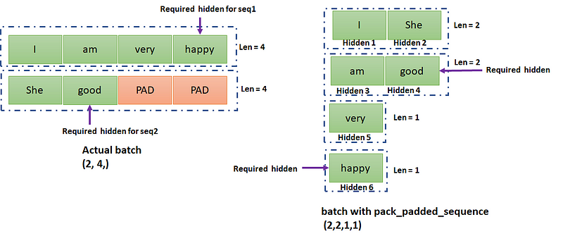
The hidden and cell need to be reset for the first token of every new sentence in LSTM and this is the reason we initialized it to zero before pass it to the LSTM. If we do not set the hidden and cell to zero Torch does it, so it is optional here. We used pack_padded_sequence and the question is why? As you remember we saw question marks in figure 3 for empty tokens, just go up if you missed them.
pack_padded_sequence
Then we used pack_padded_sequence on the embedding output. As BucketIterator grouped the similar length sequences in one batch with descending order of sequence length, and this is essential for pack_padded_sequence. The pack_padded_sequence returns you new batches from the existing batch. I will give you all the basics through code:

data: tensor([[ 6, 2, 10, 4],
             [ 9, 3, 1, 1]]) # 1 is padded token
len: tensor([4, 2])
Let’s have a batch of two sentences (1) “I am very happy” (2) “She good”. The token_ids are written above with length [4,2] The pack_padded_sequence converts the data into batches of [2, 2, 1, 1] as shown in figure 5. Let us understand this with a small example with code for that we are passing the embedding output to pack_padded_sequence with a list of seq_len we have [4, 2].
for batch in train_itr:
    text, len = batch.text
    emb = nn.Embedding(vocab_size, EMB_DIM)
    emb.weight.data.copy_(TEXT.vocab.vectors)
    emb_out = emb(text)
    pack_out = nn.utils.rnn.pack_padded_sequence(emb_out,
                                                 len,
                                                 batch_first=True)
    rnn = nn.RNN(EMB_DIM, 4, batch_first=True)
    out, hidden = rnn(pack_out)
If we print the hidden here we will get:
Hidden Output:
[[[ 0.9451, -0.9984, -0.4613,  0.9768],
         [ 0.9672, -0.9905, -0.1192,  0.9983]]]
If we print the complete output we will get:
rnn_output:
[[ 0.9092, -0.9358, -0.8513, 0.9401],
 [ 0.8691, -0.9776, 0.5006, 0.1485],
 [ 0.8109, -0.9987, 0.9487, 0.9641],
 [ 0.9672, -0.9905, -0.1192, 0.9983],
 [ 0.9926, -0.9055, -0.5543, 0.9884],
 [ 0.9451, -0.9984, -0.4613, 0.9768]]
Refer to figure 5 for this explanation (focus on purple lined tokens). The hidden of the last token will explain the sentiment for the sentence. Here is the first hidden output, that is corresponding to the last token (“happy”) of the first sequence and in rnn_output list it is the last one. The second last(5th) rnn_output is (“good”) of no use here. But the last hidden output belongs to the last token of the second sequence(“good”) and it is the 4th rnn_output. If our sequence length and data set will grow, we can save a lot of computations with pack_padded_sequence. You can transform the output to its original form of sequences by printing the following lines and I leave this part for you to analyze.
print(nn.utils.rnn.pad_packed_sequence(out, batch_first=True))
Now we have completed all the required things we need to know, we have data in our hands, we have made our model ready and we copied Glove embedding to our model’s embedding. So at last we will define some hyper-parameters then we will start training data.
Calculate Loss
opt = torch.optim.Adam(model.parameters(), lr=0.001)
criterion = nn.CrossEntropyLoss()
model.to(device)
We have defined CrossEntropyLoss (multi-class) as a loss function as we have 4 numbers of the output class and we used Adam as the optimizer. If you remember we passed the data to the device in BucketIterator so if you have Cuda then call model.to() method because data and model are to be in the same memory, either CPU or GPU. Now we will define functions to calculate the loss and accuracy of our model.
def accuracy(preds, y):
    _, preds = torch.max(preds, dim= 1)
    acc = torch.sum(preds == y) / len(y)
    return acc
def calculateLoss(model, batch, criterion):
        text, text_len = batch.text
        preds = model(text, text_len.to('cpu') )
        loss = criterion(preds, batch.label)
        acc = accuracy(preds, batch.label)
        return loss, len(batch.label), acc
The accuracy function consists of simply Torch operations: matching our predictions with actuals. In calculateLoss we passed input to our model, the only thing to note here we shifted the batch_sequence_lengths (text_len in above code) to the CPU before.
Epoch Loop
N_EPOCH = 100
for i in range(N_EPOCH):
    model.train()
    train_len, train_acc, train_loss  = 0, [], []
    for batch_no, batch in enumerate(train_itr):
        opt.zero_grad()
        loss, blen, acc = calculateLoss( model, batch,
                          criterion)
        train_loss.append(loss * blen)
        train_acc.append(acc * blen)
        train_len = train_len + blen
        loss.backward()
        opt.step()
    train_epoch_loss = np.sum(train_loss) / train_len
    train_epoch_acc = np.sum( train_acc ) / train_len
    model.eval()
    with torch.no_grad():
        for batch in val_itr:
            val_results = [calculateLoss( model, batch,
                                          criterion)
                           for batch in val_itr]
            loss, batch_len, acc = zip(*val_results)
            epoch_loss = np.sum(np.multiply(loss, batch_len))
                         / np.sum(batch_len)
            epoch_acc = np.sum(np.multiply(acc , batch_len))
                        / np.sum(batch_len)
        print('epoch:{}/{} epoch_train_loss:{:.4f},epoch_train_acc:{:.4f}'
              ' epoch_val_loss:{:.4f},epoch_val_acc:{:.4f}'.format(i+1, N_EPOCH,
                train_epoch_loss.item(), train_epoch_acc.item(),
                epoch_loss.item(), epoch_acc.item()))
If you are new to Torch: we use three important functionality (1) zero_grad to set all gradients to zero (2) loss.backward() to computes the gradients (3) opt.step() to update the parameters. All these three are only for training data so we set torch.no_grad() during evaluation phase.
Conclusion
Wow, we have completed this article, and it’s time for you to hands-on your data set. In my experience in many real-world applications, we are using sentiment analysis heavily in the industry. I hope this article helps your understanding much better than before. See you next time with some other interesting NLP article.
All the images used in this article are designed by the author.
The media shown in this article are not owned by Analytics Vidhya and are used at the Author’s discretion.


