

Machine learning models make use of randomness in obvious and unexpected ways. At a conceptual level, this non-determinism may impact your model’s convergence rate, the stability of your results, and the final quality of a network.
At a practical level, it means that you probably have difficulty reproducing the same results across runs for your model — even when you run the same script on the same training data. It could also lead to challenges in figuring out whether a change in performance is due to an actual model or data modification, or merely the result of a new random sample.
In order to tackle these sources of variation, a crucial starting point is to have full visibility into the data, model code and parameters, and details on the environment that led to a specific result. This level of reproducibility will reduce unexpected variations across your runs and help you debug machine learning experiments.
In this post, we explore areas where randomness appears in machine learning and how to achieve reproducible, deterministic, and more generalizable results by carefully setting the random seed with an example using Comet.ml.
Why is randomness important?
It may be clear that reproducibility in machine learning is important, but how do we balance this with the need for randomness? There are both practical benefits for randomness and constraints that force us to use randomness.
Practically speaking, memory and time constraints have also forced us to ‘lean’ on randomness. Gradient Descent is one of the most popular and widely used algorithms for training machine learning models, however, computing the gradient step based on the entire dataset isn’t feasible for large datasets and models. Stochastic Gradient Descent (SGD) only uses one or a mini batch of randomly picked training samples from the training set to do the update for a parameter in a particular iteration.
While SGD might lead to a noisier error in the gradient estimate, this noise can actually encourage exploration to escape shallow local minima more easily. You can take this one step farther with simulated annealing, an extension of SGD, where the model purposefully take random steps in order to seek a better state.

Randomness can also help you get more mileage out of smaller datasets with a technique called bootstrap aggregating (bagging). Most commonly seen with random forest, bagging trains multiple models on overlapping, randomly selected subset of data and
Where does randomness appear?
Now that we understand the important role that randomness plays in machine learning, we can dig into specific tasks, functions, and modeling decisions that introduce randomness.
Here are some important parts of the machine learning workflow where randomness appears:
1. Data preparation —in the case of a neural network, the shuffled batches will lead to different loss values across runs. This means your gradient values will be different across runs, and you will probably converge to a different local minima For specific types of data like time-series, audio, or text data plus specific types of models like LSTMs and RNNs, your data’s input order can dramatically impact model performance.
2. Data preprocessing —over or upsampling data to address class imbalance involves randomly selecting an observation from the minority class with replacement. Upsampling can lead to overfitting because you’re showing the model the same example multiple times.
3. Cross validation — both K-fold and Leave One Out Cross Validation (LOOCV) involve randomly splitting your data in order to evaluate the generalization performance of the model
4. Weight initialization — the initial weight values for machine learning models are often set to small, random numbers (usually in the range [-1, 1] or [0, 1]). Deep learning frameworks offer a variety of initialization methods from initializing with zeros to initializing from a normal distribution (see the Keras Initializers documentation as an example plus this excellent resource).
5. Hidden layers in the network — Dropout layers will randomly ignore a subset of nodes (each with a probability of being dropped, 1-p) during a particular forward of backward pass. This leads to differences in layer activations even when the same input is used.
6. Algorithms themselves — some models, such as random forest, are naturally dependent on randomness and others use randomness as a way of exploring the space.
Achieving Reproducibility
These factors all contribute to variations across runs — making reproducibility very difficult even if you’re working with the same model code and training data. Getting control over non-determinism and visibility into your experimentation process is crucial.
The good news is that by carefully setting the random seed across your pipeline you can achieve reproducibility. The “seed” is a starting point for the sequence and the guarantee is that if you start from the same seed you will get the same sequence of numbers. That said, you also want to test your experiments across different seed values.
We suggest a few steps to achieve both goals:
1. Use an Experiment tracking system such as Comet.ml. Given that randomness is a desirable property in experimentation, you just want to be able to reproduce the randomness as closely as possible.
2. Define a single variable that contains a static random seed and use it across your pipeline:
seed_value = 12321 # some number that you manually pick3. Report it that number to your experiment tracking system.
experiment = Experiment(project_name=”Classification model”)
experiment.log_other(“random seed”, seed_value)
4. Carefully set that seed variable for all of your frameworks:
# Set a seed value seed_value=12321# 1. Set `PYTHONHASHSEED` environment variable at a fixed value import os os.environ['PYTHONHASHSEED']=str(seed_value) # 2. Set `python` built-in pseudo-random generator at a fixed value import random random.seed(seed_value) # 3. Set `numpy` pseudo-random generator at a fixed value import numpy as np np.random.seed(seed_value) # 4. Set `tensorflow` pseudo-random generator at a fixed value import tensorflow as tf tf.set_random_seed(seed_value)
# 5. For layers that introduce randomness like dropout, make sure to set seed values
model.add(Dropout(0.25, seed=seed_value))
#6 Configure a new global `tensorflow` session
from keras import backend as K
session_conf = tf.ConfigProto(intra_op_parallelism_threads=1, inter_op_parallelism_threads=1)
sess = tf.Session(graph=tf.get_default_graph(), config=session_conf)
K.set_session(sess)

Taking these tactical measures will get you part of the way to reproducibility, but in order to have full visibility into your experiments, you’ll need to adopt a much more detailed log of your experiments.
As Matthew Rahtz describes in his blog post ‘Lessons Learned Reproducing a Deep Reinforcement Learning Paper’:
Working without a log is fine when each chunk of progress takes less than a few hours, but anything longer than that and it’s easy to forget what you’ve tried so far and end up just going in circles.
Comet.ml helps your team automatically track datasets, code changes, experimentation history, and production models — creating efficiency, transparency, and reproducibility.
Run through an example
We can put seeding to the test with Comet.ml using this example with a Keras CNN LSTM for classifying reviews from the IMDB dataset.
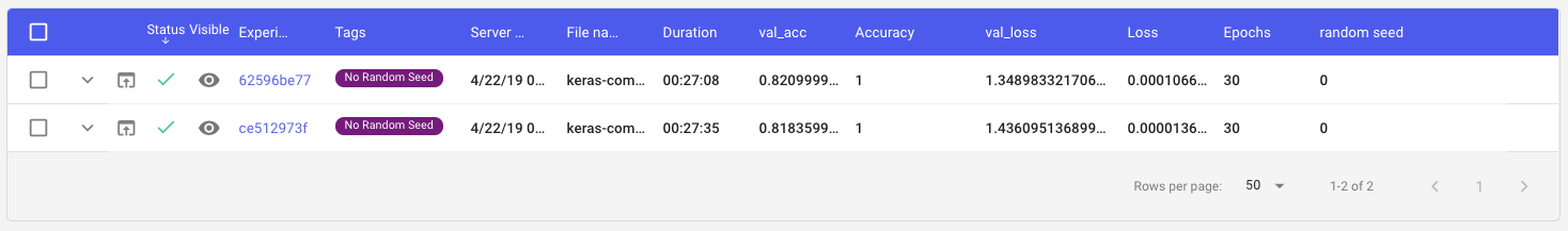
1st Round: Using the same model py file and the same IMDB training data on the same machine, we run our first two experiments and get two different validation accuracy (0.82099 vs. 0.81835) and validation loss values (1.34898 vs. 1.43609).
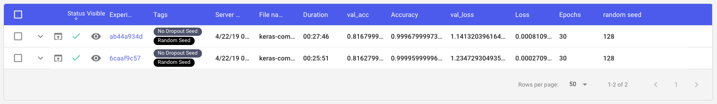
2nd Round: This time, we set the seed value for our dataset train/test split
(x_train, y_train), (x_test, y_test) = imdb.load_data(
    num_words=max_features, skip_top=50, seed=seed_value)
Even though our validation accuracy values are closer, there is still some variation between the two experiments (see the val_acc and val_losscolumns in the table below)
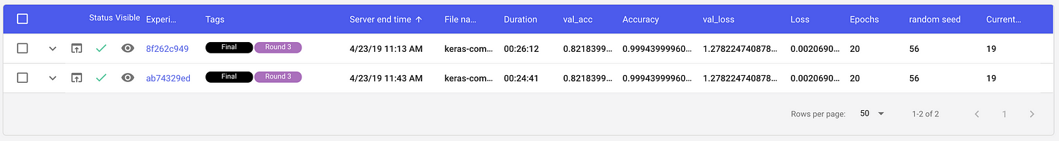
3rd Round: In addition to setting the seed value for the dataset train/test split, we will also add in the seed variable for all the areas we noted in Step 3 (above, but copied here for ease).
# Set seed value
seed_value = 56

import os
os.environ['PYTHONHASHSEED']=str(seed_value)

# 2. Set `python` built-in pseudo-random generator at a fixed value
import random
random.seed(seed_value)

# 3. Set `numpy` pseudo-random generator at a fixed value
import numpy as np
np.random.seed(seed_value)

from comet_ml import Experiment

# 4. Set `tensorflow` pseudo-random generator at a fixed value
import tensorflow as tf
tf.set_random_seed(seed_value)

# 5. Configure a new global `tensorflow` session
from keras import backend as K
session_conf = tf.ConfigProto(intra_op_parallelism_threads=1, inter_op_parallelism_threads=1)
sess = tf.Session(graph=tf.get_default_graph(), config=session_conf)
K.set_session(sess)
Now that we’ve added in our seed variables and configured a new session, the results of our experiments are finally consistently reproducible!
See the full Comet project with all the experiments we ran here
With Comet.ml, you can compare across several runs visually in real-time as training progresses:
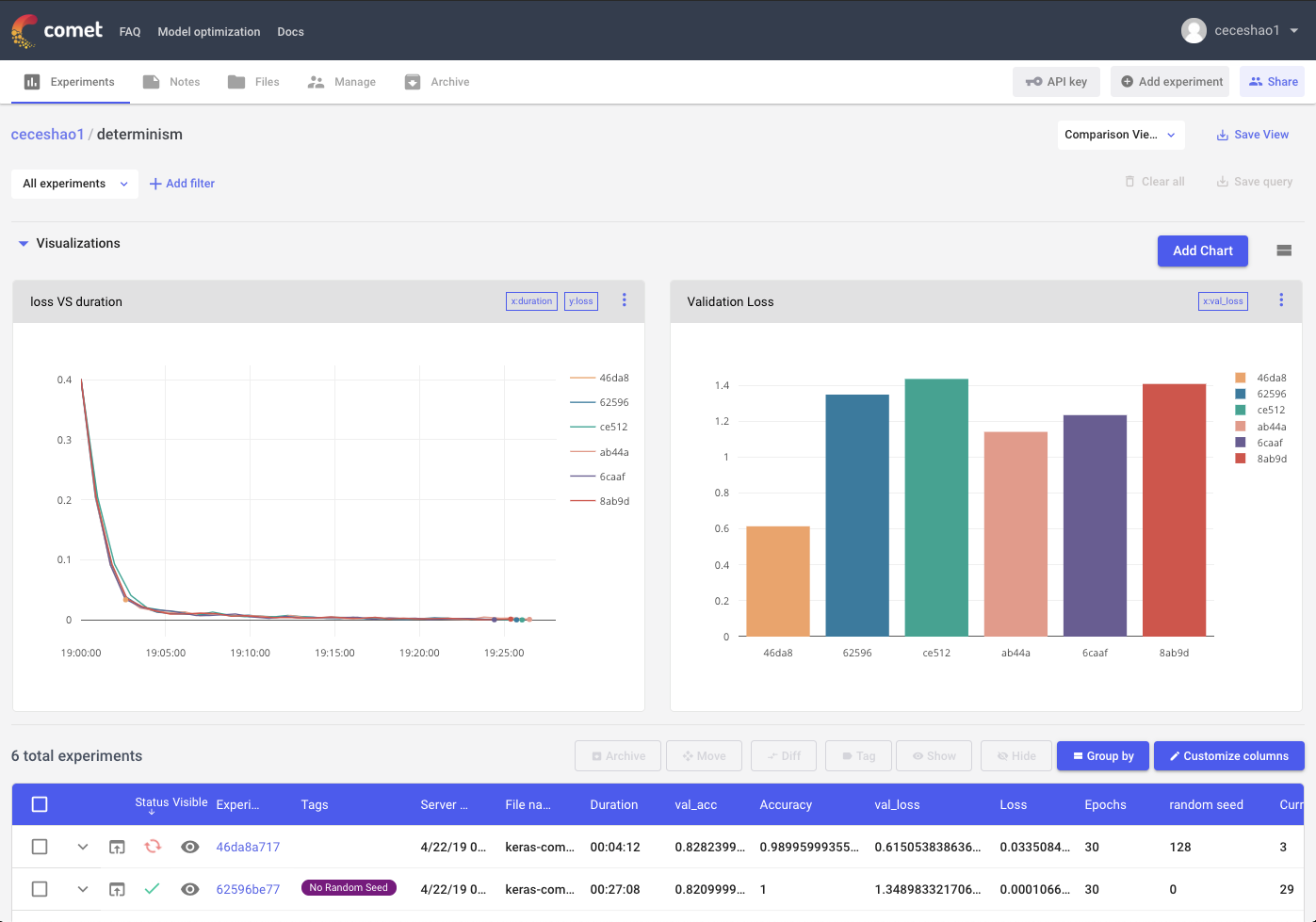
Comet helps you dig into differences in parameters, seeds, or data that might have contributed to observed changes in performance.
You can see below how one of our experiments from Round #3 specified that random seed value while one of our Round #1 experiments did not. Logging information like the random seed to Comet is flexible based on your needs.

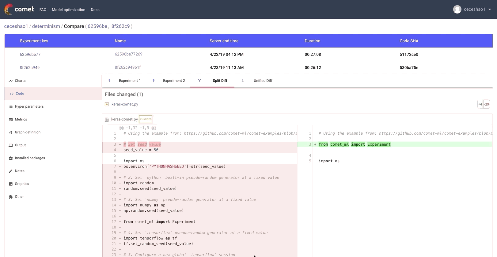
You can even inspect code differences between two experiments and see the different areas where we set our seed_value in a Round #3 experiment:
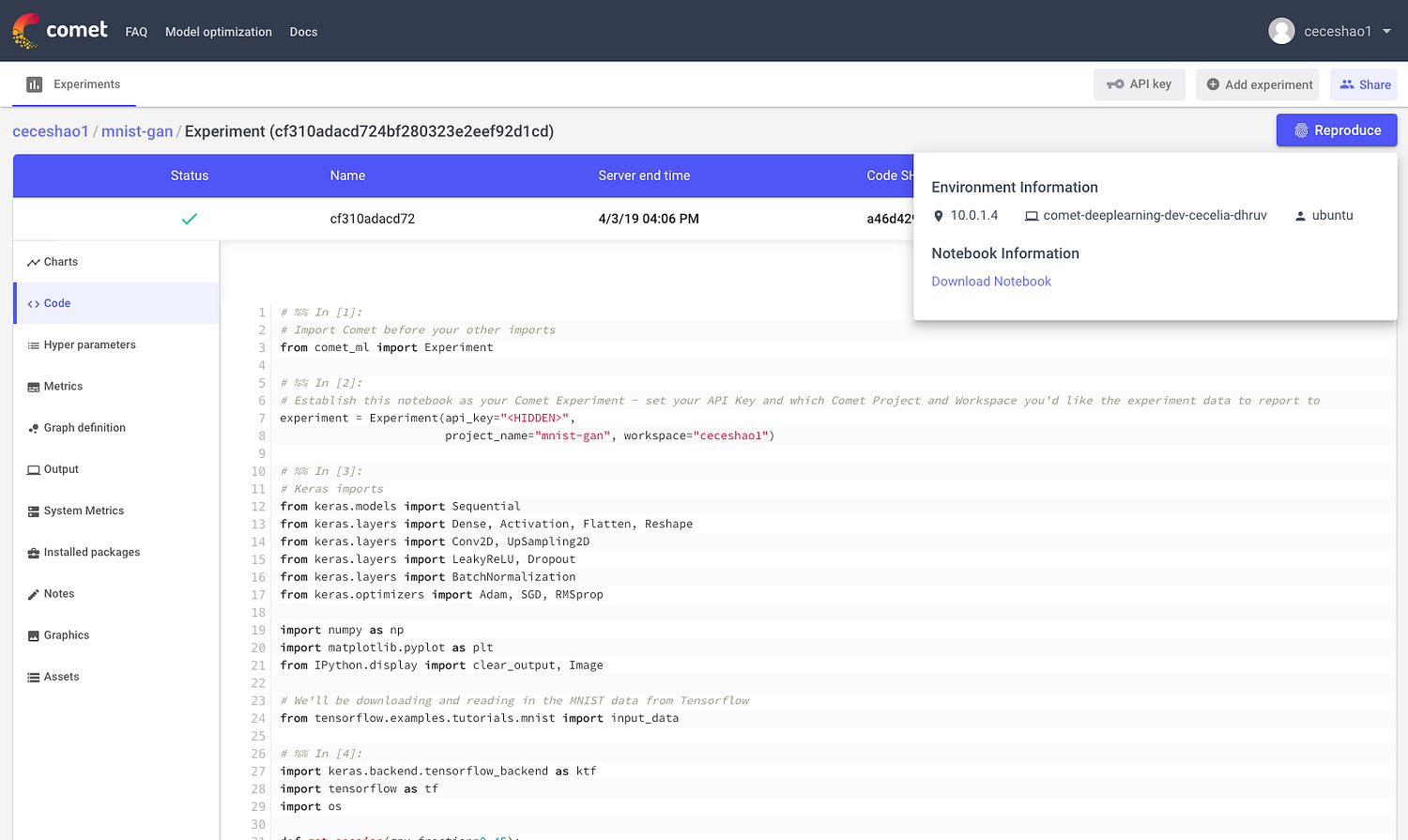
Even working with Jupyter notebooks becomes reproducible. Comet.ml shows you the code from the notebook in execution order and enables you to download the notebook that was used for the experiment with one click:
With the details for these experiments properly tracked with Comet, you can begin testing different seed values to see if those performance metrics are specific to a seed value or if your model is truly generalizable.
If you’re interested in seeing how Comet can help your data science team more productive, contact us to learn more.
Editor’s note: To learn more about Comet in person, be sure to attend Douglas Blank’s talk at ODSC East this April 30-May 4, “A Deeper Stack For Deep Learning: Adding Visualisations And Data Abstractions to Your Workflow.”