

Master Graph Algorithms for Coding Interviews
Graph algorithms can seem intimidating at first but once you understand the fundamental traversal algorithms, patterns and practice few problems, they get much easier.
In this article, we’ll cover the 10 most common Graph algorithms and patterns that appear in coding interviews, explaining how they work, when to use them, how to implement them and LeetCode problems you can practice to get better at them.
1. Depth First Search (DFS)
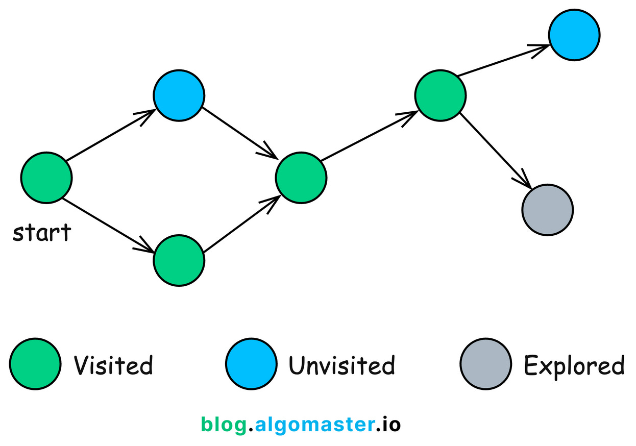
DFS is a fundamental graph traversal algorithm used to explore nodes and edges of a graph systematically.
It starts at a designated root node and explores as far as possible along each branch before backtracking.
DFS is particularly useful in scenarios like:
-
Find a path between two nodes.
-
Checking if a graph contains any cycles.
-
Identifying isolated subgraphs within a larger graph.
-
Topological Sorting: Scheduling tasks without violating dependencies.
How DFS Works:
-
Start at the Root Node: Mark the starting node as visited.
-
Explore Adjacent Nodes: For each neighbor of the current node, do the following:
-
If the neighbor hasn’t been visited, recursively perform DFS on it.
-
-
Backtrack: Once all paths from a node have been explored, backtrack to the previous node and continue the process.
-
Termination: The algorithm ends when all nodes reachable from the starting node have been visited.
Implementation:
Recursive DFS: Uses system recursion (function call stack) to backtrack.
def dfs_recursive(graph, node, visited=None):
    if visited is None:
        visited = set()
    visited.add(node)
    print(f"Visiting {node}")
    for neighbor in graph[node]:
        if neighbor not in visited:
            dfs_recursive(graph, neighbor, visited)
    return visited
Explanation:
-
Base Case: If
visitedis not provided, initialize it. -
Visit the Node: Add the current node to the
visitedset. -
Recursive Call: For each unvisited neighbor, recursively call
dfs_recursive.
Iterative DFS: Uses an explicit stack to mimic the function call behavior.
def dfs_iterative(graph, start):
    visited = set()
    stack = [start]
    while stack:
        node = stack.pop()
        if node not in visited:
            visited.add(node)
            print(f"Visiting {node}")
            # Add neighbors to stack
            stack.extend([neighbor for neighbor in graph[node] if neighbor not in visited])
    return visited
Explanation:
-
Initialize:
-
A
visitedset to keep track of visited nodes. -
A
stackwith the starting node.
-
-
Process Nodes:
-
Pop a node from the stack.
-
If unvisited, mark as visited and add its neighbors to the stack.
-
Time Complexity: O(V + E), where
Vis the number of vertices andEis the number of edges. This is because the algorithm visits each vertex and edge once.Space Complexity: O(V), due to stack used for recursion (in recursive implementation) or an explicit stack (in iterative implementation).
LeetCode Problems:
2. Breadth First Search (BFS)
BFS is a fundamental graph traversal algorithm that systematically explores the vertices of a graph level by level.
Starting from a selected node, BFS visits all of its immediate neighbors first before moving on to the neighbors of those neighbors. This ensures that nodes are explored in order of their distance from the starting node.
BFS is particularly useful in scenarios such as:
-
Finding the minimal number of edges between two nodes.
-
Processing nodes in a hierarchical order, like in tree data structures.
-
Finding people within a certain degree of connection in a social network.
How BFS Works:
-
Initialization: Create a queue and enqueue the starting node.
-
Mark the starting node as visited.
-
-
Traversal Loop: While the queue is not empty:
-
Dequeue a node from the front of the queue.
-
Visit all unvisited neighbors:
-
Mark each neighbor as visited.
-
Enqueue the neighbor.
-
-
-
Termination: The algorithm terminates when the queue is empty, meaning all reachable nodes have been visited.
Implementation:
from collections import deque

def bfs(graph, start):
    visited = set()
    queue = deque([start])
    visited.add(start)
    while queue:
        vertex = queue.popleft()
        print(f"Visiting {vertex}")
        for neighbor in graph[vertex]:
            if neighbor not in visited:
                visited.add(neighbor)
                queue.append(neighbor)
Time Complexity: O(V + E), where
Vis the number of vertices andEis the number of edges. This is because BFS visits each vertex and edge exactly once.Space Complexity: O(V) for the queue and visited set used for traversal.
LeetCode Problems:
3. Topological Sort
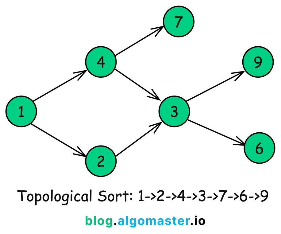
Topological Sort algorithm is used to order the vertices of a Directed Acyclic Graph (DAG) in a linear sequence, such that for every directed edge u → v, vertex u comes before vertex v in the ordering.
Essentially, it arranges the nodes in a sequence where all prerequisites come before the tasks that depend on them.
Topological Sort is particularly useful in scenarios like:
-
Determining the order of tasks while respecting dependencies (e.g., course prerequisites, build systems).
-
Figuring out the order to install software packages that depend on each other.
-
Ordering files or modules so that they can be compiled without errors due to missing dependencies.
There are two common methods to perform a Topological Sort:
1. Depth First Search (DFS) Based Algorithm:
def topological_sort_dfs(graph):
    visited = set()
    stack = []

    def dfs(vertex):
        visited.add(vertex)
        for neighbor in graph.get(vertex, []):
            if neighbor not in visited:
                dfs(neighbor)
        stack.append(vertex)

    for vertex in graph:
        if vertex not in visited:
            dfs(vertex)
    return stack[::-1]  # Reverse the stack to get the correct order
Explanation:
-
DFS Traversal: Visit each node and recursively explore its neighbors.
-
Post-Order Insertion: After visiting all descendants of a node, add it to the stack.
-
Result: Reverse the stack to obtain the topological ordering.
2. BFS-Based Topological Sort (Kahn’s Algorithm):
from collections import deque

def topological_sort_kahn(graph):
    in_degree = {u: 0 for u in graph}
    for u in graph:
        for v in graph[u]:
            in_degree[v] = in_degree.get(v, 0) + 1

    queue = deque([u for u in in_degree if in_degree[u] == 0])
    topo_order = []

    while queue:
        u = queue.popleft()
        topo_order.append(u)
        for v in graph.get(u, []):
            in_degree[v] -= 1
            if in_degree[v] == 0:
                queue.append(v)

    if len(topo_order) == len(in_degree):
        return topo_order
    else:
        raise Exception("Graph has at least one cycle")
Explanation:
-
Compute In-Degrees: Calculate the number of incoming edges for each node.
-
Initialize Queue: Start with nodes that have zero in-degree.
-
Process Nodes:
-
Dequeue a node, add it to the topological order.
-
Reduce the in-degree of its neighbors.
-
Enqueue neighbors whose in-degree becomes zero.
-
-
Cycle Detection: If the topological order doesn’t include all nodes, the graph contains a cycle.
Time Complexity: O(V + E) since each node and edge is processed exactly once.
Space Complexity: O(V) for storing the topological order and auxiliary data structures like the visited set or in-degree array.
LeetCode Problems:
4. Union Find
Union Find is a data structure that keeps track of a set of elements partitioned into disjoint (non-overlapping) subsets.
It supports two primary operations:
-
Find (Find-Set): Determines which subset a particular element belongs to. This can be used to check if two elements are in the same subset.
-
Union: Merges two subsets into a single subset, effectively connecting two elements.
Union Find is especially useful in scenarios like:
-
Quickly checking if adding an edge creates a cycle in a graph.
-
Building a Minimum Spanning Tree by connecting the smallest edges while avoiding cycles.
-
Determining if two nodes are in the same connected component.
-
Grouping similar elements together.
How Union Find Works:
The Union Find data structure typically consists of:
-
Parent Array (
parent): An array whereparent[i]holds the parent of elementi. Initially, each element is its own parent. -
Rank Array (
rank): An array that approximates the depth (or height) of the tree representing each set. Used to optimize unions.
Operations:
-
Find(x):
-
Finds the representative (root) of the set containing
x. -
Follows parent pointers until reaching a node that is its own parent.
-
Path Compression is used to optimize the time complexity of find operation, by making each node on the path point directly to the root, flattening the structure.
-
-
Union(x, y):
-
Merges the sets containing
xandy. -
Find the roots of
xandy, then make one root the parent of the other. -
Union by Rank optimization is used where the root of the smaller tree is made a child of the root of the larger tree to keep the tree shallow.
-
Implementation:
class UnionFind:
    def __init__(self, size):
        self.parent = [i for i in range(size)]  # Each node is its own parent initially
        self.rank = [0] * size  # Rank (depth) of each tree

    def find(self, x):
        if self.parent[x] != x:
            # Path compression: flatten the tree
            self.parent[x] = self.find(self.parent[x])
        return self.parent[x]

    def union(self, x, y):
        # Find roots of the sets containing x and y
        root_x = self.find(x)
        root_y = self.find(y)

        if root_x == root_y:
            # Already in the same set
            return

        # Union by rank: attach smaller tree to root of larger tree
        if self.rank[root_x] < self.rank[root_y]:
            self.parent[root_x] = root_y
        elif self.rank[root_y] < self.rank[root_x]:
            self.parent[root_y] = root_x
        else:
            # Ranks are equal; choose one as new root and increment its rank
            self.parent[root_y] = root_x
            self.rank[root_x] += 1
Time Complexity per Operation:
Find and Union: Amortized O(α(n)), where α(n) is the inverse Ackermann function, which is nearly constant for all practical purposes.
Space Complexity: O(n), where
nis the number of elements, for storing theparentandrankarrays.
LeetCode Problems:
5. Cycle Detection
Cycle Detection involves determining whether a graph contains any cycles—a path where the first and last vertices are the same, and no edges are repeated.
In other words, it’s a sequence of vertices starting and ending at the same vertex, with each adjacent pair connected by an edge.
Cycle Detection is particularly important in scenarios such as:
-
Detecting deadlocks in operating systems, to detect circular wait conditions.
-
Ensuring there are no circular dependencies in package management or build systems.
-
Understanding whether a graph is a tree or a cyclic graph.
There are different approaches for detecting cycles in graphs:
Cycle Detection in Undirected Graphs using DFS:
def has_cycle_undirected(graph):
    visited = set()

    def dfs(vertex, parent):
        visited.add(vertex)
        for neighbor in graph.get(vertex, []):
            if neighbor not in visited:
                if dfs(neighbor, vertex):
                    return True
            elif neighbor != parent:
                return True  # Cycle detected
        return False

    for vertex in graph:
        if vertex not in visited:
            if dfs(vertex, None):
                return True
    return False
Explanation:
-
DFS Traversal: Start DFS from unvisited nodes.
-
Parent Tracking: Keep track of the parent node to avoid false positives.
-
Cycle Detection Condition: If a visited neighbor is not the parent, a cycle is detected.
Cycle Detection in Directed Graphs using DFS:
def has_cycle_directed(graph):
    visited = set()
    recursion_stack = set()

    def dfs(vertex):
        visited.add(vertex)
        recursion_stack.add(vertex)
        for neighbor in graph.get(vertex, []):
            if neighbor not in visited:
                if dfs(neighbor):
                    return True
            elif neighbor in recursion_stack:
                return True  # Cycle detected
        recursion_stack.remove(vertex)
        return False

    for vertex in graph:
        if vertex not in visited:
            if dfs(vertex):
                return True
    return False
Explanation:
-
Visited Set and Recursion Stack:
-
visitedtracks all visited nodes. -
recursion_stacktracks nodes in the current path.
-
-
Cycle Detection Condition:
-
If a neighbor is in the recursion stack, a cycle is detected.
-
Cycle Detection using Union-Find (Undirected Graphs):
class UnionFind:
    def __init__(self):
        self.parent = {}

    def find(self, x):
        # Path compression
        if self.parent.get(x, x) != x:
            self.parent[x] = self.find(self.parent[x])
        return self.parent.get(x, x)

    def union(self, x, y):
        root_x = self.find(x)
        root_y = self.find(y)
        if root_x == root_y:
            return False  # Cycle detected
        self.parent[root_y] = root_x
        return True

def has_cycle_union_find(edges):
    uf = UnionFind()
    for u, v in edges:
        if not uf.union(u, v):
            return True
    return False
Explanation:
-
Initialization: Create a UnionFind instance.
-
Processing Edges:
-
For each edge, attempt to union the vertices.
-
If
unionreturnsFalse, a cycle is detected.
-
Time Complexity: O(V + E), since each node and edge is processed at most once.
Space Complexity: O(V) for the visited set and recursion stack in DFS.
LeetCode Problems:
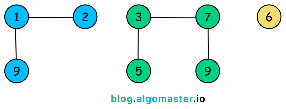
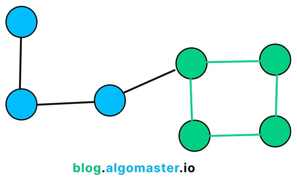
6. Connected Components
In the context of undirected graphs, a connected component is a set of vertices where each vertex is connected to at least one other vertex in the same set via some path.
Essentially, it’s a maximal group of nodes where every node is reachable from every other node in the same group.
In directed graphs, we refer to strongly connected components (SCCs), where there is a directed path from each vertex to every other vertex within the same component.
How to Find Connected Components:
We can find connected components using graph traversal algorithms like Depth-First Search (DFS) or Breadth-First Search (BFS).
The idea is to:
-
Initialize:
-
Create a
visitedset to keep track of visited nodes. -
Initialize a
componentslist to store each connected component.
-
-
Traversal:
-
For each unvisited node, perform DFS or BFS.
-
Mark all reachable nodes from this node as part of the same component.
-
Add the component to the
componentslist.
-
-
Repeat:
-
Continue the process until all nodes have been visited.
-
Implementation:
def connected_components(graph):
    visited = set()
    components = []

    def dfs(node, component):
        visited.add(node)
        component.append(node)
        for neighbor in graph.get(node, []):
            if neighbor not in visited:
                dfs(neighbor, component)

    for node in graph:
        if node not in visited:
            component = []
            dfs(node, component)
            components.append(component)

    return components
Explanation:
-
Visited Set: Keeps track of nodes that have been visited to prevent revisiting.
-
DFS Function:
-
Recursively explores all neighbors of a node.
-
Adds each visited node to the current
component.
-
-
Main Loop:
-
Iterates over all nodes in the graph.
-
For unvisited nodes, initiates DFS and collects the connected component.
-
Time Complexity: O(V + E) since each node and edge is visited exactly once.
Space Complexity: O(V) due to the
visitedset and the recursion stack (in DFS) or queue (in BFS).
Strongly Connected Components in Directed Graphs:
To find strongly connected components in a directed graph, you can use algorithms like Kosaraju’s Algorithm or Tarjan’s Algorithm.
Kosaraju’s Algorithm Steps:
-
First Pass: Perform DFS on the original graph to compute the finishing times of each node.
-
Transpose Graph: Reverse the direction of all edges.
-
Second Pass: Perform DFS on the transposed graph in the order of decreasing finishing times from the first pass.
-
Result: Each DFS traversal in the second pass identifies a strongly connected component.
LeetCode Problems:
7. Bipartite Graphs
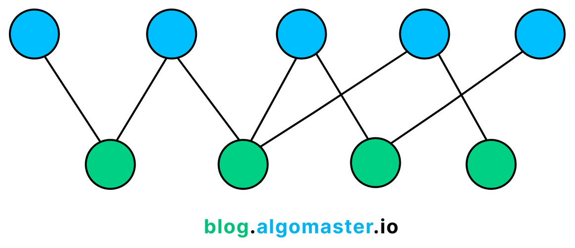
A bipartite graph is a type of graph whose vertices can be divided into two disjoint and independent sets, usually denoted as U and V, such that every edge connects a vertex from U to one in V.
In other words, no edge connects vertices within the same set.
Imagine two groups of people at a party: one group of interviewers and another of candidates. Edges represent interviews between an interviewer and a candidate. Since no interviewer interviews another interviewer and no candidate interviews another candidate, the graph naturally divides into two sets, making it bipartite.
Properties of Bipartite Graphs:
-
Two-Colorable: A graph is bipartite if and only if it can be colored using two colors such that no two adjacent vertices have the same color.
-
No Odd Cycles: Bipartite graphs do not contain cycles of odd length.
How to Check if a Graph is Bipartite:
We can determine whether a graph is bipartite by attempting to color it using two colors without assigning the same color to adjacent vertices. If successful, the graph is bipartite.
This can be done using:
-
Breadth-First Search (BFS): Assign colors level by level.
-
Depth-First Search (DFS): Assign colors recursively.
Implementation using BFS
from collections import deque

def is_bipartite(graph):
    color = {}
    for node in graph:
        if node not in color:
            queue = deque([node])
            color[node] = 0  # Assign first color
            while queue:
                current = queue.popleft()
                for neighbor in graph[current]:
                    if neighbor not in color:
                        color[neighbor] = 1 - color[current]  # Assign opposite color
                        queue.append(neighbor)
                    elif color[neighbor] == color[current]:
                        return False  # Adjacent nodes have the same color
    return True
Explanation:
-
Initialization: Create a
colordictionary to store the color assigned to each node. -
BFS Traversal: For each uncolored node, start BFS.
-
Assign the starting node a color (0 or 1).
-
For each neighbor:
-
If uncolored, assign the opposite color and enqueue.
-
If already colored and has the same color as the current node, the graph is not bipartite.
-
-
-
Result: If the traversal completes without conflicts, the graph is bipartite.
Time Complexity: O(V + E) since each node and edge is visited exactly once.
Space Complexity: O(V) due to the
colorset and the recursion stack (in DFS) or queue (in BFS).
LeetCode Problems:
8. Flood Fill
Flood Fill is an algorithm that determines and alters the area connected to a given node in a multi-dimensional array.
Starting from a seed point, it finds or fills (or recolors) all connected pixels or cells that have the same color or value.
How Flood Fill Works:
-
Starting Point: Begin at the seed pixel (starting coordinates).
-
Check the Color: If the color of the current pixel is the target color (the one to be replaced), proceed.
-
Replace the Color: Change the color of the current pixel to the new color.
-
Recursively Visit Neighbors:
-
Move to neighboring pixels (up, down, left, right—or diagonally, depending on implementation).
-
Repeat the process for each neighbor that matches the target color.
-
-
Termination: The algorithm ends when all connected pixels of the target color have been processed.
Implementation
Recursive Flood Fill:
def flood_fill_recursive(image, sr, sc, new_color):
    rows, cols = len(image), len(image[0])
    color_to_replace = image[sr][sc]
    if color_to_replace == new_color:
        return image

    def dfs(r, c):
        if (0 <= r < rows and 0 <= c < cols and image[r][c] == color_to_replace):
            image[r][c] = new_color
            # Explore neighbors: up, down, left, right
            dfs(r + 1, c)  # Down
            dfs(r - 1, c)  # Up
            dfs(r, c + 1)  # Right
            dfs(r, c - 1)  # Left

    dfs(sr, sc)
    return image
Explanation:
-
Base Case: If the color to replace is the same as the new color, return the image as is.
-
DFS Function:
-
Checks bounds and whether the current pixel matches the color to replace.
-
Changes the color of the current pixel.
-
Recursively calls itself on adjacent pixels.
-
Iterative Flood Fill:
from collections import deque

def flood_fill_iterative(image, sr, sc, new_color):
    rows, cols = len(image), len(image[0])
    color_to_replace = image[sr][sc]
    if color_to_replace == new_color:
        return image

    queue = deque()
    queue.append((sr, sc))
    image[sr][sc] = new_color

    while queue:
        r, c = queue.popleft()
        for dr, dc in [(-1, 0), (1, 0), (0, -1), (0, 1)]:  # Directions: up, down, left, right
            nr, nc = r + dr, c + dc
            if (0 <= nr < rows and 0 <= nc < cols and image[nr][nc] == color_to_replace):
                image[nr][nc] = new_color
                queue.append((nr, nc))

    return image
Explanation:
-
Initialization:
-
Use a
dequeas a queue to manage pixels to process. -
Start by enqueuing the seed pixel.
-
-
Processing Loop:
-
Dequeue a pixel.
-
For each direction (up, down, left, right), check if the neighbor needs to be filled.
-
If so, change its color and enqueue it.
-
-
Termination:
-
The loop ends when there are no more pixels to process.
-
Time Complexity: O(N), where N is the number of pixels in the area to be filled. Each pixel is visited at most once.
Space Complexity:
Recursive Implementation: O(N), due to the call stack in recursion.
Iterative Implementation: O(N), if using a queue or stack to manage pixels.
LeetCode Problems:
9. Minimum Spanning Tree
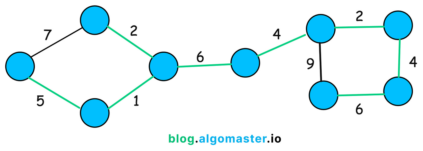
An MST is a subset of the edges of a connected, undirected, weighted graph that connects all the vertices together, without any cycles, and with the minimum possible total edge weight.
In simpler terms, it’s the cheapest possible way to connect all nodes in a network without any loops.
Key Algorithms for Finding MSTs:
1. Kruskal’s Algorithm:
-
Builds the MST by adding edges incrementally, starting with the smallest.
-
Uses Union Find data structure to detect cycles.
Implementation:
class UnionFind:
    def __init__(self, size):
        self.parent = [i for i in range(size)]
        self.rank = [0] * size

    def find(self, x):
        if self.parent[x] != x:
            # Path compression
            self.parent[x] = self.find(self.parent[x])
        return self.parent[x]

    def union(self, x, y):
        root_x = self.find(x)
        root_y = self.find(y)
        if root_x == root_y:
            return False  # Cycle detected
        # Union by rank
        if self.rank[root_x] < self.rank[root_y]:
            self.parent[root_x] = root_y
        elif self.rank[root_y] < self.rank[root_x]:
            self.parent[root_y] = root_x
        else:
            self.parent[root_y] = root_x
            self.rank[root_x] += 1
        return True

def kruskal_mst(num_nodes, edges):
    # edges is a list of tuples: (weight, node_u, node_v)
    uf = UnionFind(num_nodes)
    mst = []
    total_weight = 0

    # Sort edges based on weight
    edges.sort(key=lambda x: x[0])

    for weight, u, v in edges:
        if uf.union(u, v):
            mst.append((u, v, weight))
            total_weight += weight
            print(f"Edge added: ({u}, {v}) with weight {weight}")
        else:
            print(f"Edge ({u}, {v}) with weight {weight} creates a cycle and is skipped.")

    print(f"Total weight of MST: {total_weight}")
    return mst
Explanation:
-
UnionFind Class:
-
Manages disjoint sets to detect cycles efficiently.
-
-
Edge Sorting:
-
Edges are sorted by weight to consider the smallest edges first.
-
-
Main Loop:
-
Iterates over sorted edges.
-
Attempts to union the sets containing the edge’s vertices.
-
If union is successful, the edge is added to the MST.
-
If it would create a cycle, the edge is skipped.
-
Time Complexity: O(E log E) since sorting edges takes O(E log E) and union find operations are nearly constant time
Space Complexity: O(V + E), O(V) for storing the parent and rank arrays in union find and O(E) for storing the edges.
2. Prim’s Algorithm:
-
Starts from an arbitrary node and grows the MST by adding the cheapest edge from the tree to a new vertex.
import heapq

def prim_mst(graph, start=0):
    num_nodes = len(graph)
    visited = [False] * num_nodes
    min_heap = [(0, start, -1)]  # (weight, current_node, parent_node)
    mst = []
    total_weight = 0

    while min_heap and len(mst) < num_nodes - 1:
        weight, u, parent = heapq.heappop(min_heap)
        if not visited[u]:
            visited[u] = True
            if parent != -1:
                mst.append((parent, u, weight))
                total_weight += weight
                print(f"Edge added: ({parent}, {u}) with weight {weight}")

            for v, w in graph[u]:
                if not visited[v]:
                    heapq.heappush(min_heap, (w, v, u))

    if len(mst) != num_nodes - 1:
        print("Graph is not connected.")
        return None

    print(f"Total weight of MST: {total_weight}")
    return mst
Explanation:
-
Initialization:
-
visitedarray tracks visited nodes. -
min_heapis a priority queue initialized with the starting node.
-
-
Main Loop:
-
While the heap is not empty and the MST is incomplete:
-
Pop the edge with the minimum weight.
-
If the node hasn’t been visited:
-
Mark it as visited.
-
Add the edge to the MST (if it’s not the starting node).
-
Add all edges from this node to the heap.
-
-
-
-
Termination:
-
The algorithm ends when all nodes are included in the MST.
-
Checks if the MST spans all nodes (graph is connected).
-
Time Complexity: O(E log V) using a priority queue (min-heap).
Space Complexity: O(V) for the priority queue and arrays used.
LeetCode Problems:
10. Shortest Path
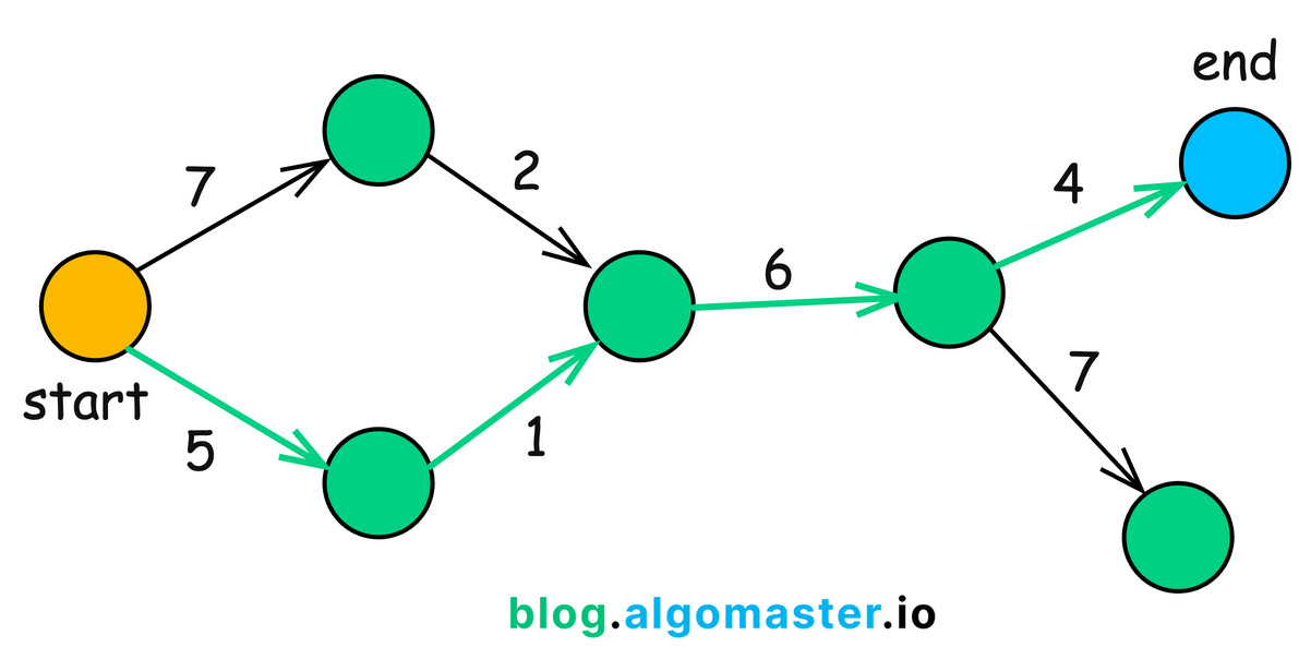
The Shortest Path problem involves finding the path between two vertices (nodes) in a graph such that the sum of the weights of its constituent edges is minimized.
In simpler terms, it’s about finding the most efficient route from a starting point to a destination in a network.
Key Algorithms for Finding Shortest Paths:
1. Dijkstra’s Algorithm:
-
Finds the shortest paths from a single source vertex to all other vertices in a graph with non-negative edge weights.
-
It’a a greedy algorithm that uses a priority queue (min-heap).
import heapq

def dijkstra(graph, start):
    # graph: adjacency list where graph[u] = [(v, weight), ...]
    distances = {vertex: float('inf') for vertex in graph}
    distances[start] = 0
    priority_queue = [(0, start)]
    while priority_queue:
        current_distance, current_vertex = heapq.heappop(priority_queue)
        # Skip if we have found a better path already
        if current_distance > distances[current_vertex]:
            continue
        for neighbor, weight in graph[current_vertex]:
            distance = current_distance + weight
            # If a shorter path to neighbor is found
            if distance < distances[neighbor]:
                distances[neighbor] = distance
                heapq.heappush(priority_queue, (distance, neighbor))
    return distances
Explanation:
-
Initialization:
-
distancesdictionary stores the shortest known distance to each vertex. -
priority_queueis a min-heap storing(distance, vertex)tuples.
-
-
Main Loop:
-
Pop the vertex with the smallest known distance.
-
For each neighbor, calculate the new distance.
-
If the new distance is shorter, update and push onto the heap.
-
-
Result:
-
Returns the shortest distances from the start vertex to all other vertices.
-
Time Complexity: O(V + E log V) using a min-heap (priority queue).
Space Complexity: O(V) for storing distances and the priority queue.
2. Bellman-Ford Algorithm:
-
Computes shortest paths from a single source vertex to all other vertices, even when the graph has negative edge weights.
-
It can detect negative cycles.
def bellman_ford(graph, start):
    # graph: list of edges [(u, v, weight), ...]
    num_vertices = len({u for edge in graph for u in edge[:2]})
    distances = {vertex: float('inf') for edge in graph for vertex in edge[:2]}
    distances[start] = 0

    # Relax edges repeatedly
    for _ in range(num_vertices - 1):
        for u, v, weight in graph:
            if distances[u] + weight < distances[v]:
                distances[v] = distances[u] + weight

    # Check for negative-weight cycles
    for u, v, weight in graph:
        if distances[u] + weight < distances[v]:
            raise Exception("Graph contains a negative-weight cycle")

    return distances
Explanation:
-
Initialization:
distancesdictionary stores the shortest known distance to each vertex. -
Main Loop: Iterate
num_vertices - 1times, relaxing all edges. -
Negative Cycle Check: A final pass to check for improvements indicates a negative cycle.
-
Result: Returns the shortest distances from the start vertex to all other vertices.
Time Complexity: O(V * E)
Space Complexity: O(V) for storing distances.
3. Breadth-First Search (BFS):
-
Applicable for unweighted graphs or graphs where all edges have the same weight.
-
Finds the shortest path by exploring neighbor nodes level by level.
from collections import deque

def bfs_shortest_path(graph, start, target):
    visited = set()
    queue = deque([(start, [start])])  # Each element is a tuple (node, path_to_node)
    visited.add(start)

    while queue:
        current_node, path = queue.popleft()

        if current_node == target:
            return path  # Shortest path found

        for neighbor in graph[current_node]:
            if neighbor not in visited:
                visited.add(neighbor)
                queue.append((neighbor, path + [neighbor]))

    return None  # Path not found
4. A* (A-Star) Algorithm:
-
Used for graphs where you have a heuristic estimate of the distance to the target.
-
Commonly used in pathfinding and graph traversal, especially in games and AI applications.
How It Works:
-
A* combines features of Dijkstra’s Algorithm and Greedy Best-First Search.
-
It selects the path that minimizes
f(n) = g(n) + h(n), where:-
g(n)is the actual cost from the start node to the current noden. -
h(n)is the heuristic estimated cost fromnto the goal.
-
Implementation:
import heapq

def a_star(graph, start, goal, heuristic):
    open_set = []
    heapq.heappush(open_set, (0 + heuristic(start, goal), 0, start, [start]))  # (f_score, g_score, node, path)
    closed_set = set()

    while open_set:
        f_score, g_score, current_node, path = heapq.heappop(open_set)

        if current_node == goal:
            return path  # Shortest path found

        if current_node in closed_set:
            continue
        closed_set.add(current_node)

        for neighbor, weight in graph[current_node]:
            if neighbor in closed_set:
                continue
            tentative_g_score = g_score + weight
            tentative_f_score = tentative_g_score + heuristic(neighbor, goal)
            heapq.heappush(open_set, (tentative_f_score, tentative_g_score, neighbor, path + [neighbor]))

    return None  # Path not found
Time Complexity:
Worst-case: O(b^d), where b is the branching factor (average number of successors per state) and d is the depth of the solution.
Best-case: O(d), when the heuristic function is perfect and leads directly to the goal.
Space Complexity: O(b^d), as it needs to store all generated nodes in memory.
5. Floyd-Warshall Algorithm:
-
Computes shortest paths between all pairs of vertices.
-
Suitable for dense graphs with smaller numbers of vertices.
-
The algorithm iteratively updates the shortest paths between all pairs of vertices by considering all possible intermediate vertices.
Implementation:
def floyd_warshall(graph):
    # Initialize distance and next_node matrices
    nodes = list(graph.keys())
    dist = {u: {v: float('inf') for v in nodes} for u in nodes}
    next_node = {u: {v: None for v in nodes} for u in nodes}

    # Initialize distances based on direct edges
    for u in nodes:
        dist[u][u] = 0
        for v, weight in graph[u]:
            dist[u][v] = weight
            next_node[u][v] = v

    # Floyd-Warshall algorithm
    for k in nodes:
        for i in nodes:
            for j in nodes:
                if dist[i][k] + dist[k][j] < dist[i][j]:
                    dist[i][j] = dist[i][k] + dist[k][j]
                    next_node[i][j] = next_node[i][k]

    # Check for negative cycles
    for u in nodes:
        if dist[u][u] < 0:
            raise Exception("Graph contains a negative-weight cycle")

    return dist, next_node
Time Complexity: O(V^3)
Space Complexity: O(V^2) for storing the distance array.
LeetCode Problems:
Thank you for reading!
If you found it valuable, hit a like ❤️ and consider subscribing for more such content every week.
If you have any questions or suggestions, leave a comment.
P.S. If you’re finding this newsletter helpful and want to get even more value, consider becoming a paid subscriber.
As a paid subscriber, you’ll receive an exclusive deep dive every week, access to a comprehensive system design learning resource , and other premium perks.
There are group discounts, gift options, and referral bonuses available.
Checkout my Youtube channel for more in-depth content.
Follow me on LinkedIn, X and Medium to stay updated.
Checkout my GitHub repositories for free interview preparation resources.
I hope you have a lovely day!
See you soon,
Ashish