This article was published as a part of the Data Science Blogathon.
Introduction
Linear programming, also called mathematical programming, is a branch of mathematics that we use to solve a system of linear equations or inequalities to maximize or minimize some linear function.
The objective is to find the optimal values of the objective function, which is why this problem statement is also known as Linear Optimization, where we optimize the solutions while simultaneously minimizing or maximizing the objective function.
Discrete Optimization & Solving Techniques
With this, let us take a step back and understand what Discrete Optimization is! Discrete optimization is a part of optimization methodology that deals with discrete quantities, i.e., non-continuous functions. Familiarity with such optimization techniques is of paramount importance for data scientists & Machine Learning practitioners as discrete and continuous optimization problems lie at the heart of modern ML and AI systems as well as data-driven business analytics processes. The resolutions of the problems within this domain lie in the techniques of Linear programming(as defined above) & Mixed-Integer Linear Programming.
We use Mixed-Integer linear programming in solving problems with at least one of the variables ( for now, consider these as the independent variables of any equation) that is discrete rather than being continuous. On the surface level, it might seem that it is better to have discrete values rather than continuous real numbers, right?

Unfortunately not! I shall answer this question after outlining some basic terminologies in Linear programming for a coherent understanding.
Basic Terminologies of Linear Programming
Consider a small linear programming problem below: –
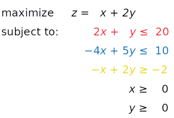
The motive here is to find out the optimal values of x & y such that the inequalities are given in red, blue & yellow, and inequalities x ≥ 0 and y ≥ 0 are satisfied. The optimal values are those that maximize the objective function(z).
Objective Function – It is also known as the cost function or the “goal” of our optimization problem. Either we’ll maximize or minimize it based on the given problem statement. For example, it could be maximizing the profit of a company or minimizing the expenses of the company due to its regular functioning.
Decision Variables –The independent variables to be found to optimize the objective function are called the decision variables. In this case, x and y are the decision variables that are the unknowns of the mathematical programming model.
Constraints – The restrictions on the decision variables in an optimization problem are known as constraints. In the above example, the inequalities in red, blue & yellow are the constraints. Note that these could very well be equations or equality constraints.
Non – negativity restrictions – The limitation on the decision variables that they will lie in the first quadrant only or their values could not be less than zero are known as the non-negative constraints. Here x, y >= 0 are the non-negative constraints
Feasible Region – A feasible region or solution space is the set of all possible points of an optimization problem that satisfy the problem’s constraints. Let us understand the feasible region with the help of visualization of the constraints given in the example: –
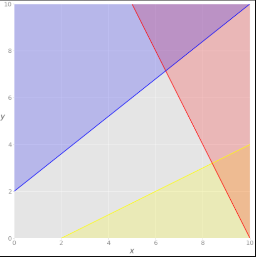
There is a red area above the red line that implies the inequality 2x + y = 20 is unsatisfactory. In the same way, the blue area violates the blue inequality because it is the function -4x + 5y = 10. The yellow line is −x + 2y = −2, and the yellow area below it is where the yellow inequality isn’t valid. Each point of the gray area satisfies all constraints and is a potential solution to the problem. This area is called the feasible region, and its points are feasible solutions. In this case, there’s an infinite number of feasible solutions. That’s also known as the Graphical Method. For a better understanding of this method, please refer to the video.
Now that we are familiar with the terminologies let us throw some more light on Mixed-Linear integer programming. This type of problem is important, especially when we express quantities in integers like the number of products produced by the machine or the number of customers served. Mixed-integer linear programming allows for overcoming many demerits of linear programming. One can approximate non-linear functions with piecewise linear functions, model-logical constraints (a yes/no problem like whether a customer will churn or not), and more. A piecewise linear function is a segmented real-valued function where the graph consists of line segments only & the data follows a different linear trend over different regions of data. We would not go into the details of it but you could read more about it here.
Now, remember a question that arises whether or not discrete values are better than continuous values -let us take that up. So, integer programming, as the name suggests, compels some or all of the variables to assume only integer values. Hence, integer variables make an optimization problem non-convex, and therefore, far more difficult to solve.
Why does Convexity matter?
A convex optimization problem is a problem where all of the constraints are convex functions, and the objective is a convex function if minimizing or a concave function if maximizing. Linear functions are convex, so linear programming problems are convex problems.
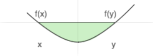
A function is called convex- if a line segment is drawn from any point (x, f(x)) to another point (y, f(y)), from x to y — lies on or above the graph of f, as shown in the figure below.
Source: Author
For a convex function, it is just opposite – line segment lies on or below the graph of the function f. This is only possible as the values in [x, y] are continuous.
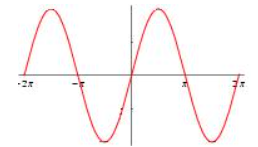
But if the values are discrete – in the case of integer programming – then it leads to a non-convex optimization problem. A non-convex function “curves up and down” — it is neither convex nor concave, as shown in the figure below.
Source: Author
Non-convex optimization may have multiple locally optimal points, and it can take a lot of time to identify whether the problem has no solution or if the solution is global. Hence, the efficiency of the convex optimization problem in time is much better. Memory and solution time may rise exponentially as you add more integer variables. If you wish to dive deeper into mathematics, then please go through this article.
Unbounded and Infeasible Linear Programming
Till now, we have just discussed feasible linear programming problems because they have bounded feasible regions and finite solutions. But we might come across problems where the feasible regions are not bounded, or the problem is infeasible.

Source: https://realpython.com/linear-programming-python/
Infeasible LP – A linear programming problem is infeasible if it doesn’t have a solution. This usually happens when no solution can satisfy all constraints at once.
For example, consider adding an inequality constraint (x + y <= -3) in the above-given example with color-coded inequalities. In this case, one of the decision variables has to be negative right? This would consequently violate the non-negative constraints. Such a system doesn’t have a feasible solution, so it’s called infeasible.
Unbounded Solution – A linear programming problem is unbounded if its feasible region isn’t bounded and the solution is not finite. This means that at least one of your variables isn’t constrained and can reach up to positive or negative infinity, making the objective infinite as well.
For example, if we’ll remove red and yellow inequalities, then we can’t bound decision variables on the positive end. This would make the decision variables (x or y) limitless and the objective function infinite as well.
Solvers
There are several suitable and great Python tools for linear programming and mixed-integer linear programming problems. Some of them are open source, while others are proprietary. Almost all widely used linear programming and mixed-integer linear programming libraries are native to and written in Fortran or C or C++. This is because linear programming requires computationally intensive work with (often large) matrices. Such libraries are called solvers. The Python tools are just wrappers around the solvers. Think of it as Numpy in Python, which provides a C-API to enable users to get access to the array objects.
Also, note that there are many optimizer tools for solving LP problems like TORA. But, the knowledge of performing optimization programmatically is second to none! So we should have an excellent knowledge of that too.
Implementation in Code
Now, I know you must be tired of the theoretical concepts and would probably need a “Well deserved” break. Familiarity with the foundational concepts is important, but do not fret. We will now straight away jump to a Resource Allocation Problem and will look into its implementation in Python. Several free Python libraries are also available for interacting with linear or mixed-integer linear programming solvers, including the following: –
For this article, we shall be using PuLP for tackling the LPP.
Problem
Suppose you are a dietician and is responsible to advise one of your customer on the best possible food plan he should follow to attain “optimum nutrition”.
In addition, you’ll have to consider some restrictions like budget and the variety of food. You can download the data set from here and the jupyter notebook from my Github repository.
Intuition
Minimize the cost of the best food plan(inclusive of food items), given some constraints (on total calories but also each of the nutritional components, e.g., fat, vitamin C, iron, etc.).
The Cost function is the total cost of the food items, which we are trying to minimize. Why? Because the cost should be minimal, at the same time, deriving the nutritional value from the combination of different food items should be maximum, considering the maximum and minimum constraints given in the data. A nutritional component’s minimum and maximum bounds define the inequality constraints.
You can install PuLP using Pip and then import everything from the library.
pip install pulp
#If directly running on Jupyter then you could use the following: -
!pip3 install pulp
#Import everything from the library
from pulp import *

import numpy as np, pandas as pd

import warnings

warnings.filterwarnings('always')

warnings.filterwarnings('ignore')
Formulation of the Optimization Problem
First, we create an LP problem using the method LpProblem in PuLP.
prob = LpProblem('Diet_Problem', LpMinimize)
Now, we read the data set and create some dictionaries to extract information from the diet table. Note we are reading only the first 17 rows with the “nrows=17” argument because we just want to read all the nutrients’ information and not the maximum/minimum bounds in the dataset. We will enter those bounds in the optimization problem separately.
df = pd.read_excel('diet.xls',nrows=17)
df.head() #Here we see the data

Source: Author
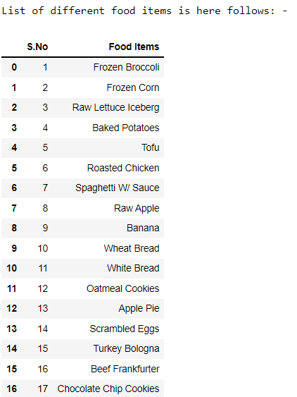
Now we create a list of all the food items and thereafter create dictionaries of these food items with all the remaining columns. The columns denote the nutrition components or the decision variables here. Apart from the price per serving and the serving quantity, all the other columns denote the nutritional components like fat, Vitamins, cholesterol, etc. In this optimization problem, the minimum and maximum intakes of nutritional components are specified, which serve as constraints.
food = list(df.Foods)
#The list of items
count=pd.Series(range(1,len(food)+1))
print('List of different food items is here follows: -')
food_s = pd.Series(food)
#Convert to data frame
f_frame = pd.concat([count,food_s],axis=1,keys=['S.No','Food Items'])
f_frame
Source: Author
Now we create dictionaries of the food items with each of the nutritional components.
# Create a dictinary of costs for all food items
costs = dict(zip(food,df['Price/Serving']))
#Create a dictionary of calories for all items of food
calories = dict(zip(food,df['Calories']))
#Create a dictionary of cholesterol for all items of food
chol = dict(zip(food,df['Cholesterol (mg)']))
#Create a dictionary of total fat for all items of food
fat = dict(zip(food,df['Total_Fat (g)']))
#Create a dictionary of sodium for all items of food
sodium = dict(zip(food,df['Sodium (mg)']))
#Create a dictionary of carbohydrates for all items of food
carbs = dict(zip(food,df['Carbohydrates (g)']))
#Create a dictionary of dietary fiber for all items of food
fiber = dict(zip(food,df['Dietary_Fiber (g)']))
#Create a dictionary of protein for all food items
protein = dict(zip(food,df['Protein (g)']))
#Create a dictionary of vitamin A for all food items
vit_A = dict(zip(food,df['Vit_A (IU)']))
#Create a dictionary of vitamin C for all food items
vit_C = dict(zip(food,df['Vit_C (IU)']))
#Create a dictionary of calcium for all food items
calcium = dict(zip(food,df['Calcium (mg)']))
#Create a dictionary of iron for all food items
iron = dict(zip(food,df['Iron (mg)']))
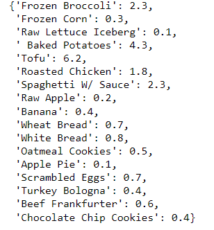
We just observe one of these dictionaries to see what it looks like. Here we take the example of ‘iron’ with all the food items in the data.
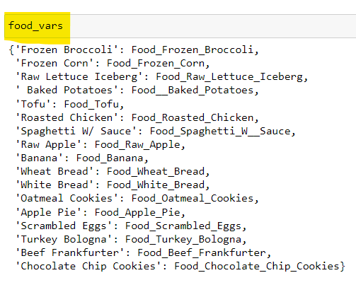
We now create a dictionary of all the food items’ variables keeping the following things in mind: –
- The lower bound is equal to zero
- The category should be continuous i.e. the decision variables could take continuous values.
Such adjustment is necessary to enable the non-negative conditions as anyway negative quantities of food is not possible right? Imagine -1 block of tofu -would not make any sense at all! Furthermore, it ensures that the values have a real value.
# A dictionary called 'food_vars' is created to contain the referenced Variables
food_vars = LpVariable.dicts("Food",food,lowBound=0,cat='Continuous')
Objective Function Addition
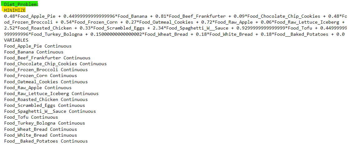
prob += lpSum([costs[i]*food_vars[i] for i in food])
prob
We build the linear programming problem by adding the main objective function. Note the use of the lpSum method. Note – we have the optimum solution for our problem and the output given below indicates the same.
Source: Author
Addition of the Constraints
Note that we further put our constraints now based upon the maximum and the minimum intake of the nutritional components in our data set. Do not forget the motive, we intend to minimize the cost considering these constraints on the components or the decision variables.
For the sake of simplicity, and to maintain brevity, I am planning to define only five constraints. Now the lpSum method helps in calculating the sum of the linear expressions, so we will use it to define the constraint of Calories in the data.
lpSum([food_vars[i]*calories[i] for i in food])

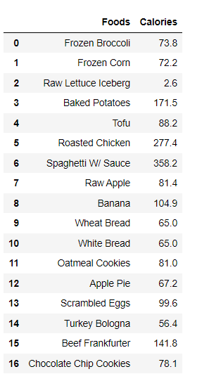
Hence in the two output images above, we could compare that lpSum helps in taking the sum-product of the food items with their respective size of the nutritional component taken under consideration (Calories in this case)
Note that we still have not defined the constraints. We define it by adding the same to our problem statement (Recall the objective function and the constraints are part of the LPP)
prob += lpSum([food_vars[x]*calories[x] for x in food]) >= 800, "CaloriesMinimum"
prob += lpSum([food_vars[x]*calories[x] for x in food]) <= 1300, "CaloriesMaximum"
prob
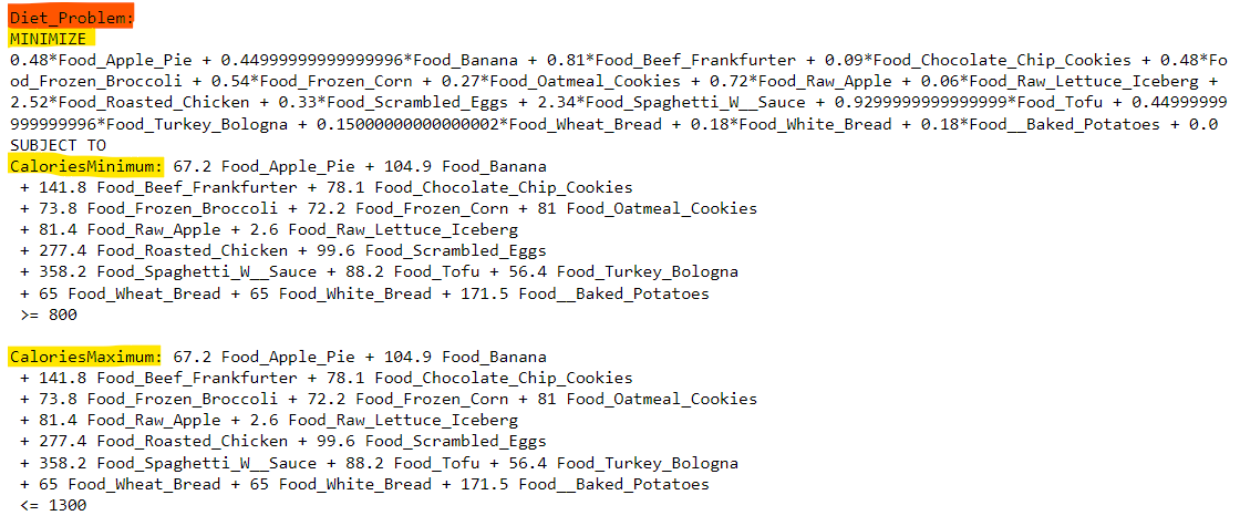
Hence, the output shows how beautifully the function works. We have the objective function which is subject to the “Calories” constraint as defined in the code above. After the definition of one of the five components of nutrition, let’s move ahead and define the four remaining components as well to formulate the problem.
The five nutritional components that I have chosen are Carbohydrates, Fat, Protein, Vitamin A & Calcium.
#Carbohydrates' constraint
prob += lpSum([food_vars[x]*carbs[x] for x in food]) >= 130, "CarbsMinimum"
prob += lpSum([food_vars[x]*carbs[x] for x in food]) <= 200, "CarbsMaximum"
#Fat's constraint
prob += lpSum([food_vars[x]*fat[x] for x in food]) >= 20, "FatsMinimum"
prob += lpSum([food_vars[x]*fat[x] for x in food]) <= 50, "FatsMaximum"
#Protein's constraint
prob += lpSum([food_vars[x]*protein[x] for x in food]) >= 100, "ProteinsMinimum"
prob += lpSum([food_vars[x]*protein[x] for x in food]) <= 150, "ProteinsMaximum"
#Vit_A constraint
prob += lpSum([food_vars[x]*vit_A[x] for x in food]) >= 1000, "Vit_A_Minimum"
prob += lpSum([food_vars[x]*vit_A[x] for x in food]) <= 10000, "Vit_A_Maximum"
This concludes the formulation of the LPP. The most significant part is the building up of the problem statement with the objective function and the constraints defined correctly. The solving is just a cakewalk (at least in programming!)
Running the Solver Algorithm
Finally, we have our problem ready and now we shall run the Solver algorithm. Note that we could pass parameters to the solver when running it, but in this case, I will run it without any parameters and let it determine the best algorithm to run based on the structure of the problem. Yes, this library is quite optimal to do so!
prob.solve()
PuLP allows you to choose solvers and formulate problems more naturally. The default solver used by PuLP is the COIN-OR Branch and Cut Solver (CBC). It will connect to the COIN-OR Linear Programming Solver (CLP) for linear relaxations.
prob. solver
>>
Now we print the status of the problem. Note that if we don’t formulate the problem well, then it might have an “infeasible” solution, or if it does not provide sufficient information, then it might be “Unbounded”. But our solution is “optimal”, which means that we have optimum values.
LpStatus[prob.status]
>> ‘Optimal’
You can get the optimization results as the attributes of the model. The function value() and the corresponding method .value() return the actual values of the attributes. prob.objective holds the value of the objective function, prob.constraints contains the values of the slack variables (we don’t require them but just a good to know fact).
for var in prob.variables():
    print(f'Variable name: {var.name} , Variable value : {var.value()}n')
print('n')
print('*'*100)
print('n')
#We can also see the slack variables of the constraints
for name, con in prob.constraints.items():
    print(f'constraint name:{name}, constraint value:{con.value()}n')
print('*'*100)
print('n')
## OBJECTIVE VALUE
print(f'OBJECTIVE VALUE IS: {prob.objective.value()}')
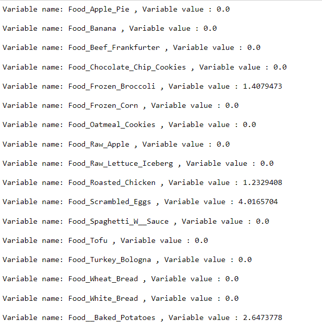
Decision Variables’ optimized values
Source: Author
Value of the Objective Function
The optimal value of the objective function is $5.58. The interpretation of the result would be the following: –
2.64 servings of baked potatoes
4.02 servings of scrambled eggs
1.23 servings of Roasted chicken
1.41 servings of Frozen broccoli
Conclusion
So, with the optimal value, we have charted out a diet plan that minimizes the budget (cost of the diet plan) and maximizes the nutritional components for the individual.
- The key takeaway here is that we could attain the best outcome basis linear inequalities (or equalities) through the optimization technique described above.
- Kindly note that you could get the optimization problems in different ways. For example, imagine you have a business strategy and some business practices that when applied might lead to a significant increase in profits. Hence, your job, in this case, is to maximize the profitability of the business by selecting the best strategies out of the available strategies.
- Another example could be a factory production plan. Each machine has a maximum production capacity and it produces different items with different characteristics. As an engineer, your job would be to ensure the maximum output of the items considering all the capacity constraints of the machinery.
Endnotes
Since we did not mention any parameter hence the PuLP uses the default solver CBC for the resolution. We could have used a different solver for our solution such as GNU Linear Programming Kit(GLPK). Some well-known and very powerful commercial and proprietary solutions are Gurobi, CPLEX, and XPRESS.
I hope I was able to give you some concrete idea of how we go about solving Linear programming problems using PuLP. If you think any portion is ambiguous or needs improvement, you are most welcome to make suggestions. Thank you for reading!
About the Author
Hi there! Currently, I am working as a credit analyst in the field of Finance after pursuing a Bachelor’s degree in Statistics.
My areas of interest include Data Science, ML/DL, Statistics, and BI/Analytics. Please feel free to reach out to me on LinkedIn and have a look at some of my other projects on my Github profile. You could also connect with me via mail for absolutely anything!
The media shown in this article is not owned by Analytics Vidhya and are used at the Author’s discretion.


