This article was published as a part of the Data Science Blogathon
Hello readers. This is part-1 of a comprehensive tutorial on Linear predictive models. I am writing this article mostly for beginners, and since there is a lot to cover, all the topics will be divided into a few articles. The articles will have a practical code-based approach so one can easily start coding after reading this one article. Let us begin.
Contents
1) Linear Prediction Models
2) Importing libraries and loading data
3) Getting familiar with the data
4) Data Cleaning and Preparation
5) Exploratory Data Analysis
- Correlation heatmap
6) One-Hot Encoding and K-folds
7) Modeling
- Linear Regression
- Linear Regression with regularization
- Linear Regression with Regu, Pipeline, and Cross Val Predict
- Linear Regression with Polynomial Regularization
8) What to expect in the next part
Linear Prediction Models
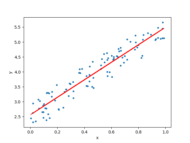
Linear prediction modeling has applications in a number of fields like data forecasting, speech recognition, low-bit-rate coding, model-based spectral analysis, interpolation, signal restoration, etc. These linear algorithms have their origin from statistics, and in the statistical literature, these models are referred to as autoregressive (AR) processes. We will explore some of the types of linear regression like Lasso, Ridge, etc in the next articles. In this article, we will cover Linear regression with and without regularization, regression using Regu, pipeline, Cross Val Predict, etc.
For this series of articles, we have scraped data from the website AutoScout24 and acquired the dataset for used cars sale from Germany. You can find the extracted dataset here. The notebook for this article is linked at the end of this article, be sure to check that out.
Importing Libraries and loading data
First, we import the necessary libraries:
import os
import pandas as pd
import numpy as np
import seaborn as sns
import matplotlib.pyplot as plt

from pandas_profiling import ProfileReport
import warnings
warnings.filterwarnings("ignore")
Our aim is to predict the prices of the car based on the data scraped.
Getting familiar with the data
df.shape
> (46405, 9)
df.describe()

df['fuel'].unique()

df['gear'].unique()
> array(['Manual', 'Automatic', nan, 'Semi-automatic'], dtype=object)
df.info()
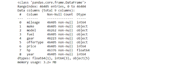
Thus there are a few values in our dataset. Since the amount seems very low, we can hopefully omit them. We’ll tackle this in the next section:
Data Cleaning and Preparation
df.isna().sum()

Since the amount of missing values is less than 1% of our total data, I presume we can drop these entries without any problems.
df.dropna(inplace = True)
#dropping duplicate rows
df.drop_duplicates(keep = 'first', inplace = True)
#now let's see the shape of our dataframe df.shape
> (43947, 9)
df.describe()

We can use the column Year to generate the age of a particular vehicle which can be more helpful for our predictions. For this, we use the DateTime module.
from datetime import datetime
df['age'] = datetime.now().year - df['year']
df.drop('year',axis = 1, inplace = True)
df.head()

Exploratory Data Analysis
M = df.price.median()
print(M)
> 10990.0
m = df.price.mean()
print(m)
> 16546.56379275036
below_M = df.query("price<10990")
no_below_M = below_M.value_counts().sum()

above_M = df.query("price > 10990.1")
no_above_M = above_M.value_counts().sum()

print(f'Median = {M}')
print('Number of cars with values above the median')
print(no_above_M)
print('Number of cars with values below the median')
print(no_below_M)
print('--------------------------------------------')

below_m = df.query("price<16546")
no_below_m = below_m.value_counts().sum()

above_m = df.query("price > 16546.1")
no_above_m = above_m.value_counts().sum()

print(f'Median = {m}')
print('Number of cars with values above the mean')
print(no_above_m)
print('Number of cars with values below the mean')
print(no_below_m)

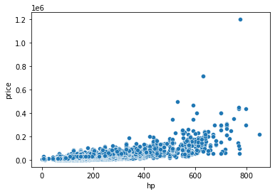
sns.scatterplot(x=df['hp'], y=df['price'])
#Changing the fuels from categorical values to integer values
df['fuel'] = df['fuel'].replace('Diesel', 0)
df['fuel'] = df['fuel'].replace('Gasoline', 1)
df['fuel'] = df['fuel'].replace(['Electric/Gasoline', 'Electric/Diesel', 'Electric'],  2)
df['fuel'] = df['fuel'].replace(['CNG', 'LPG', 'Others', '-/- (Fuel)', 'Ethanol', 'Hydrogen'], 3)
Correlation Heatmap
plt.figure(figsize=(14,7))
sns.heatmap(df.corr(),annot=True, cmap='coolwarm')

Now we try to find the popular cars, i.e the cars that are more affordable and give better mileage and more people can buy.
min_price, max_price = df.price.quantile([0.01, 0.99])
min_price, max_price
> (3300.0, 83468.84000000004)
pop_cars = df[(df.pricemin_price)]
print('Total number of cars:')
print(df.shape[0]) print('---------------------')
print('Numers of cars that are abore $3.300,0 and below $99.999,0')
print(pop_cars.shape[0])

min_price, max_price = df.mileage.quantile([0.01, 0.99])
min_price, max_price
> (7.0, 259170.56000000006)
pop_cars = pop_cars[(pop_cars.mileagemin_price)]
min_price, max_price = df.hp.quantile([0.01, 0.999])
min_price, max_price
> (60.0, 650.0)
pop_cars = pop_cars[(pop_cars.hpmin_price)]
Changing the fuel type back to categorical values and resetting the index:
pop_cars['fuel'] = pop_cars['fuel'].replace(0, 'Diesel')
pop_cars['fuel'] = pop_cars['fuel'].replace(1, 'Gasoline')
pop_cars['fuel'] = pop_cars['fuel'].replace(2, 'Electric')
pop_cars['fuel'] = pop_cars['fuel'].replace(3, 'Others')
pop_cars = pop_cars.reset_index(drop=True)
One-Hot Encoding and K-folds
pop_cars = pop_cars.drop(columns=['make', 'model'], axis=1)
pop_cars.head()

pop_cars.dtypes.value_counts()
> object     3
  int64      3
  float64    1
  dtype: int64
mask = pop_cars.dtypes == np.object
categorical = pop_cars.columns[mask]
categorical
> Index(['fuel', 'gear', 'offerType'], dtype='object')
num_ohc_cols = (pop_cars[categorical].apply(lambda x: x.nunique()).sort_values(ascending=False))
num_ohc_cols
> offerType    5
  fuel         4
  gear         3
  dtype: int64
from sklearn.preprocessing import OneHotEncoder, LabelEncoder

data_ohc = pop_cars.copy()
ohc = OneHotEncoder()

for col in num_ohc_cols.index:
  #this is a sparse array
  new_dat = ohc.fit_transform(data_ohc[[col]])
  #drop original column from original DF
  data_ohc = data_ohc.drop(col, axis=1)
  #get unique names of columns
  cats = ohc.categories_
  #create a column for each OHE column by value
  new_cols = ['_'.join([col,cat]) for cat in cats[0]]
  #create the new Dataset
  new_df = pd.DataFrame(new_dat.toarray(), columns=new_cols)
  #append new data to df
  data_ohc=pd.concat([data_ohc, new_df], axis=1)

y_col = 'price'
feature_cols = [x for x in data_ohc.columns if x != y_col]
X = data_ohc[feature_cols]
y = data_ohc[y_col]
from sklearn.model_selection import KFold
kf = KFold(shuffle=True, random_state=72018, n_splits=3)
kf.split(X)
This creates a Tuple, for 3 different scenarios(n_plits), that is: train_index, test_index
for train_index, test_index in kf.split(X):
  print("Train index:", train_index[:10], len(train_index))
  print("Test index:", test_index[:10], len(test_index))
  print('')

Modeling
Everything we did until this point, is to prepare our data for modeling. Now we will implement various types of Linear Regression and see which model has the most accuracy.
1) Linear Regression
from sklearn.linear_model import LinearRegression
from sklearn.metrics import r2_score, mean_squared_error

scores = []
lr = LinearRegression()

for train_index, test_index in kf.split(X):
  X_train, X_test, y_train, y_test = (X.iloc[train_index, :], X.iloc[test_index, :], y[train_index], y[test_index])

  lr.fit(X_train, y_train)

  y_pred = lr.predict(X_test)

  score = r2_score(y_test.values, y_pred)

  scores.append(score)

scores
> [0.8287930876292234, 0.8297633896297357, 0.8390539858927717]
2) Linear Regression with Regularization
from sklearn.preprocessing import StandardScaler

scores = []
lr = LinearRegression()
s = StandardScaler()

for train_index, test_index in kf.split(X):
  X_train, X_test, y_train, y_test = (X.iloc[train_index, :], X.iloc[test_index, :], y[train_index], y[test_index])

  X_train_s = s.fit_transform(X_train)

  lr.fit(X_train_s, y_train)

  X_test_s = s.transform(X_test)

  y_pred = lr.predict(X_test_s)

  score = r2_score(y_test.values, y_pred)

  scores.append(score)

scores
> [0.8287665996258867, 0.829763389629736, 0.8390557075678731]
3) Linear Regression with Regu, Pipeline, and Cross Val Predict
# doing what we did above with Pipeline
from sklearn.pipeline import Pipeline

estimator = Pipeline([('scaler', s), ('linear_reg', lr)])

estimator.fit(X_train, y_train)

estimator.predict(X_test)

kf
> KFold(n_splits=3, random_state=72018, shuffle=True)
from sklearn.model_selection import cross_val_predict
predictions = cross_val_predict(estimator, X, y, cv=kf, verbose=100)
r2_score(y, predictions)
> 0.8326247491666151
We can see that this is almost the same. Linear Regression doesn’t change much with Regularization
4) Linear Regression with Polynomial Regularization
from sklearn.preprocessing import PolynomialFeatures
from sklearn.model_selection import KFold

powers = [2, 3, 4]
lr1 = LinearRegression()
scores = []

for power in powers:
  pf = PolynomialFeatures(power)
  estimator = Pipeline([('make_higher_degree', pf), ('linear_reg', lr1)])
  predictions = cross_val_predict(estimator, X, y, cv=kf, verbose=100)
  score = r2_score(y, predictions)
  scores.append(score)

list(zip(powers, scores))
> [(2, 0.8834636269383815), (3, 0.816677589576142), (4, -1026.6737588070525)]
Thus we can see that a polynomial regression with an exponent of 2, is the one with the highest accuracy of 88.3%.
What to expect in the next part
There are a few more linear algorithms like lasso, ridge, GridSearchCV that I’d like to cover in the next article. Using these more advanced and complicated algorithms might give us a more accurate prediction than 88%. We might even touch the 90-mark. be sure to look out for the next article once it is published. You can find it here:
Barney6, Author at Analytics Vidhya
Here is the Github link for the code for this article:

