This article was published as a part of the Data Science Blogathon
Introduction
In computer vision, we have a convolutional neural network that is very popular for computer vision tasks like image classification, object detection, image segmentation and a lot more.
Image classification is one of the most needed techniques in today’s era, it is used in various domains like healthcare, business, and a lot more, so knowing and making your own state of the art computer vision model is a must if you’re in a domain of AI.
In this article, We will learn from basics to advanced concepts covering CNN and then we will build a model that classifies an image as a cat or a dog using Tensorflow, then we will learn about Advanced computer vision in which we will cover Transfer learning and we will build a multi-image classifier using Convolutional Neural Networks ( CNN ).
Convolution Neural Network
A convolutional neural network ( CNN ) is a type of neural network for working with images, This type of neural network takes input from an image and extract features from an image and provide learnable parameters to efficiently do the classification, detection and a lot more tasks.
We extract the features from the images using something called “filters”, we have different filters used to extract different features from the images.
Let’s take an example, you are building a classification model which detects whether an image is of cat or non-cat. So we have different filters used to extract different features from an image like in this case, one filter may learn to detect the eyes of a cat another learn to detect ears and etc.

How do we extract the information using these filters?
We convolute our image using filters using convolution operations, Confused??, let’s see in detail with some visualization.
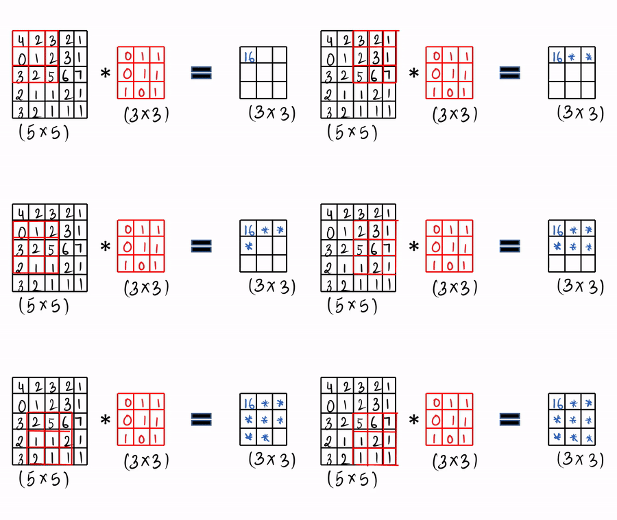
Given:- We take our image ( 5 x 5 ), here we have greyscale image and then we take our learnable filters ( 3 x3 ) and then we do the convolution operation.

Step:1:- You do the element wise product and then you sum it all up and then you fill the first cell. [ 4 * 0 + 1 * 2 + 1 * 3 + 0 * 0 + 1 * 1 + 2 * 1 + 3 * 1 + 2 * 0 + 5 * 1 = 16 ]

Then you slide by a factor of 1 and again you do the same thing which is called the convolution operation by just doing element-wise product and sum it up.
You can see the visualization in GIF format.
You may ask a question how can we do for RGB scale or colourful image, you have to do the same instead of your number of channels.
1.) Stride Convolutions:-
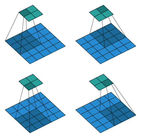
In the above examples, we are sliding over our images with the factor of 1, so for faster computation over the images, so in the below example we are sliding over the image with the factor of 2.
2.) Padding:-
In convolution operation, we often lose some information, so for preserving the information, we pad our image with zeros and then we start convoluting our image.
3.) Pooling Layer:-
In order to downsample images while preserving information, we use pooling layers, we have two types of pooling layers which are max-pooling and average pooling.

In the above image, we are doing max-pooling, and also if you want to use average pooling then you can take average instead of max.
4.) Upsampling layer:-
In order to upsample or make your image large you use these types of layers, it often sometimes blur your image or other disadvantages.
5.) Get to know the dimensions:- After your image is convoluted then how you will get to know the dimension, so here is the formula for calculating the dimension of your image after convoluting:-
((n-f+2p)/s) + 1
- n is the size of the input, if you have a 32x32x3 image then n will be 32.
- f is the size of the filer, if your size of the filter is 3×3, then f will be 3.
- p is the padding.
- s is the factor by which you want to slide
That’s it for knowing about CNN, I hope that you understood CNN, we will build a full CNN for classification and a lot more.
Image Classification
Image Classification:- It’s the process of extracting information from the images and labelling or categorizing the images. There are two types of classification:-
- Binary classification:- In this type of classification our output is in binary value either 0 or 1, let’s take an example that you’re given an image of a cat and you have to detect whether the image is of cat or non-cat.
- Multi-class classification:- In this type of classification our output will be multi-class, so let’s take an example that you’re given an image and you have to detect the breed of dog among 37 classes.
Building a Cat and Dog Image Classifier using CNN
Problem Statement:- We are given an image and we need to make a model that classifies whether that image is of a cat or dog.
Dataset:- I am using the cat and dog dataset from kaggle, you can find the link here.
Approach:- Github link.
Step:- 1) Importing the necessary libraries
import numpy as np
import pandas as pd
import os
from pathlib import Path
import glob

import seaborn as sns
import matplotlib.pyplot as plt

import tensorflow as tf
from tensorflow.keras import layers
from tensorflow.keras import Model
from tensorflow.keras.optimizers import RMSprop
from keras_preprocessing.image import ImageDataGenerator
Step:- 2) Loading the data and basic EDA
data_dir = Path('../input/cat-and-dog') # data directory
train_dir = data_dir / "training_set/training_set"
test_dir = data_dir / "test_set/test_set"
cat_samples_dir_train = train_dir / "cats" # directory for cats images
dog_samples_dir_train = train_dir / "dogs" # directory for dogs images
def make_csv_with_image_labels(CATS_PATH, DOGS_PATH):

    '''

    Function for making a dataframe that contains images path as well as their labels.

    Parameters:-

     - CATS_PATH - Path for Cats  Images

     - DOGS_PATH - Path for Dogs Images

    Output:-

    It simply returns dataframe

    '''

    cat_images = CATS_PATH.glob('*.jpg')

    dog_images = DOGS_PATH.glob('*.jpg')

    df = []

    for i in cat_images:

        df.append((i, 0)) # appending cat images as 0

    for j in dog_images:

        df.append((i, 1)) # appending dog images as 0

    df = pd.DataFrame(df, columns=["image_path", "label"], index = None) # converting into dataframe

    df = df.sample(frac = 1).reset_index(drop=True)

    return df

train_csv = make_csv_with_image_labels(cat_samples_dir_train,dog_samples_dir_train)

train_csv.head()
Now, we will visualize the number of images for each class.
len_cat = len(train_csv["label"][train_csv.label == 0])
len_dog = len(train_csv["label"][train_csv.label == 1])
arr = np.array([len_cat , len_dog])
labels = ['CAT', 'DOG']
print("Total No. Of CAT Samples :- ", len_cat)
print("Total No. Of DOG Samples :- ", len_dog)
plt.pie(arr, labels=labels, explode = [0.2,0.0] , shadow=True)
plt.show()
Step:- 3) Preparing the training and testing data
def get_train_generator(train_dir, batch_size=64, target_size=(224, 224)):
    '''
    Function for preparing training data
    '''
    train_datagen = ImageDataGenerator(rescale = 1./255., # normalizing the image
                                   rotation_range = 40,
                                   width_shift_range = 0.2,
                                   height_shift_range = 0.2,
                                   shear_range = 0.2,
                                   zoom_range = 0.2,
                                   horizontal_flip = True)
    train_generator = train_datagen.flow_from_directory(train_dir,
                                                    batch_size = batch_size,
                                                    color_mode='rgb',
                                                    class_mode = 'binary',
                                                    target_size = target_size)
    return train_generator
train_generator = get_train_generator(train_dir)
Output :- Found 8005 images belonging to 2 classes.
Now, we will prepare the testing data,
def get_testgenerator(test_dir,batch_size=64, target_size=(224,224)):
    '''
    Function for preparing testing data
    '''
    test_datagen = ImageDataGenerator( rescale = 1.0/255. )
    test_generator  =  test_datagen.flow_from_directory(test_dir,
                                                          batch_size  = batch_size,
                                                          color_mode='rgb',
                                                          class_mode  = 'binary',
                                                          target_size = target_size)
    return test_generator
test_generator = get_testgenerator(test_dir)
Output:- Found 2023 images belonging to 2 classes.
Step:- 4) Building the Model
Now, we will start building our model, below is the full architecture implemented in Tensorflow. We will start with a convolution block with 64 filters, with the kernel size of (3×3) and stride of 2 followed by relu activation layer.
and then we will proceed in the same way by changing filters and at last we have added 4 dense or FC layers, as this is the binary classification so, our last activation layer is sigmoid.
model = tf.keras.Sequential([
    layers.Conv2D(64, (3,3), strides=(2,2),padding='same',input_shape= (224,224,3),activation = 'relu'),
    layers.MaxPool2D(2,2),
    layers.Conv2D(128, (3,3), strides=(2,2),padding='same',activation = 'relu'),
    layers.MaxPool2D(2,2),
    layers.Conv2D(256, (3,3), strides=(2,2),padding='same',activation = 'relu'),
    layers.MaxPool2D(2,2),
    layers.Flatten(),
    layers.Dense(158, activation ='relu'),
    layers.Dense(256, activation = 'relu'),
    layers.Dense(128, activation = 'relu'),
    layers.Dense(1, activation = 'sigmoid'),
])
model.summary()

Building the Model
Step:- 5) Compile and Train the Model
model.compile(optimizer=RMSprop(lr=0.001), loss='binary_crossentropy', metrics=['acc'])
history = model.fit_generator(train_generator,
                              epochs=15,
                              verbose=1,
                              validation_data=test_generator)

Step:- 6) Evaluating the model
import matplotlib.image  as mpimg
import matplotlib.pyplot as plt
acc=history.history['acc']
val_acc=history.history['val_acc']
loss=history.history['loss']
val_loss=history.history['val_loss']
epochs=range(len(acc))
plt.plot(epochs, acc, 'r', "Training Accuracy")
plt.plot(epochs, val_acc, 'b', "Validation Accuracy")
plt.title('Training and validation accuracy')
plt.figure()
plt.plot(epochs, loss, 'r', "Training Loss")
plt.plot(epochs, val_loss, 'b', "Validation Loss")
plt.title('Training and validation loss')
model.save('my_model.h5') # saving the trained model

new_model = tf.keras.models.load_model('./my_model.h5') # loading the trained model
Transfer Learning
The basic intuition behind transfer learning is you take a pre-trained model that is already trained on a larger dataset with a lot of extensive hyperparameter tuning, and you fine-tune this model on your data just by removing some top layers.
It helps you to transfer knowledge from one model to another. You can see here how we implement this here.
Endnotes
Thanks for reading! I hope that you’ll implement these concepts & strategies into ML projects. Something not mentioned or want to share your thoughts? Feel free to comment below And I’ll get back to you.
About the Author
Ayush Singh
I am a 14-year-old learner and machine learning and deep learning practitioner, Working in the domain of Natural Language Processing, Generative Adversarial Networks, and Computer Vision. Also, make videos on machine learning, deep learning, Gans on my youtube channel Newera. I am also a competitive coder but still practising all the techs and a passionate learner and educator. You can connect me on Linkedin:- Ayush Singh

