Introduction
Over the last 12 months, I have been participating in a number of machine learning hackathons on Analytics Vidhya and Kaggle competitions. After the competition, I always make sure to go through the winner’s solution. The winner’s solution usually provide me critical insights, which have helped me immensely in future competitions.
Most of the winners rely on an ensemble of well-tuned individual models along with feature engineering. If you are starting with machine learning, I would advise you to lay emphasis on these two areas as I have found them equally important to do well in a machine learning.
Most of the time, I was able to crack the feature engineering part but probably didn’t use the ensemble of multiple models. If you are a beginner, it’s even better to get familiar with ensembling as early as possible. Chances are that you are already applying it without knowing!
In this article, I’ll take you through the basics of ensemble modeling. Then I will walk you through the advantages of ensembling. Also, to provide you hands-on experience on ensemble modeling, we will use ensembling on a hackathon problem using R.
Table of Content
- What is ensembling?
- Types of ensembling
- Advantages and disadvantages of ensembling
- Practical guide to implementing ensembling in R
- Additional resources
P.S. For this article, we will assume that you can build individual models in R / Python. If not, you can start your journey with our learning path.
1.What is ensembling?
In general, ensembling is a technique of combining two or more algorithms of similar or dissimilar types called base learners. This is done to make a more robust system which incorporates the predictions from all the base learners. It can be understood as conference room meeting between multiple traders to make a decision on whether the price of a stock will go up or not.
Since all of them have a different understanding of the stock market and thus a different mapping function from the problem statement to the desired outcome. Therefore, they are supposed to make varied predictions on the stock price based on their own understandings of the market.
Now we can take all of these predictions into account while making the final decision. This will make our final decision more robust, accurate and less likely to be biased. The final decision would have been opposite if one of these traders would have made this decision alone.
You can consider another example of a candidate going through multiple rounds of job interviews. The final decision of candidate’s ability is generally taken based on the feedback of all the interviewers. Although a single interviewer might not be able to test the candidate for each required skill and trait. But the combined feedback of multiple interviewers usually helps in better assessment of the candidate.
2. Types of ensembling
Some of the basic concepts which you should be aware of before we go into further detail are:
- Averaging: It’s defined as taking the average of predictions from models in case of regression problem or while predicting probabilities for the classification problem.
- Majority vote: It’s defined as taking the prediction with maximum vote / recommendation from multiple models predictions while predicting the outcomes of a classification problem.
- Weighted average: In this, different weights are applied to predictions from multiple models then taking the average which means giving high or low importance to specific model output.
Practically speaking, there can be a countless number of ways in which you can ensemble different models. But these are some techniques that are mostly used:
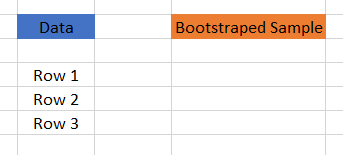
- Bagging: Bagging is also referred to as bootstrap aggregation. To understand bagging, we first need to understand bootstrapping. Bootstrapping is a sampling technique in which we choose ‘n’ observations or rows out of the original dataset of ‘n’ rows as well. But the key is that each row is selected with replacement from the original dataset so that each row is equally likely to be selected in each iteration. Let’s say we have 3 rows numbered 1, 2 and 3.
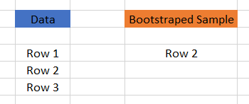
For bootstrapped sample, we choose one out of these three randomly. Say we chose Row 2.
You see that even though Row 2 is chosen from the data to the bootstrap sample, it’s still present in the data. Now, each of the three:
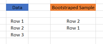
Rows have the same probability of being selected again. Let’s say we choose Row 1 this time.
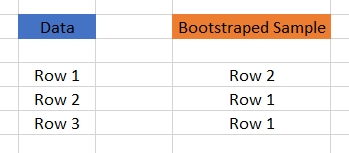
Again, each row in the data has the same probability to be chosen for Bootstrapped sample. Let’s say we randomly choose Row 1 again.
Thus, we can have multiple bootstrapped samples from the same data. Once we have these multiple bootstrapped samples, we can grow trees for each of these bootstrapped samples and use the majority vote or averaging concepts to get the final prediction. This is how bagging works.
One important thing to note here is that it’s done mainly to reduce the variance. Now, random forest actually uses this concept but it goes a step ahead to further reduce the variance by randomly choosing a subset of features as well for each bootstrapped sample to make the splits while training.
- Boosting: Boosting is a sequential technique in which, the first algorithm is trained on the entire dataset and the subsequent algorithms are built by fitting the residuals of the first algorithm, thus giving higher weight to those observations that were poorly predicted by the previous model.
It relies on creating a series of weak learners each of which might not be good for the entire dataset but is good for some part of the dataset. Thus, each model actually boosts the performance of the ensemble.
It’s really important to note that boosting is focused on reducing the bias. This makes the boosting algorithms prone to overfitting. Thus, parameter tuning becomes a crucial part of boosting algorithms to make them avoid overfitting.
Some examples of boosting are XGBoost, GBM, ADABOOST, etc.
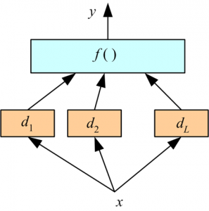
- Stacking: In stacking multiple layers of machine learning models are placed one over another where each of the models passes their predictions to the model in the layer above it and the top layer model takes decisions based on the outputs of the models in layers below it.
Let’s understand it with an example:
Here, we have two layers of machine learning models:
- Bottom layer models (d1, d2, d3 ) which receive the original input features(x) from the dataset.
- Top layer model, f() which takes the output of the bottom layer models (d1, d2, d3 ) as its input and predicts the final output.
- One key thing to note here is that out of fold predictions are used while predicting for the training data.
Here, we have used only two layers but it can be any number of layers and any number of models in each layer. Two of the key principles for selecting the models:
- The individual models fulfill particular accuracy criteria.
- The model predictions of various individual models are not highly correlated with the predictions of other models.
One thing that you might have realized is that we have used the top layer model which takes as input the predictions of the bottom layer models. This top layer model can also be replaced by many other simpler formulas like:
- Averaging
- Majority vote
- Weighted average
3. Advantages and Disadvantages of ensembling
3.1 Advantages
- Ensembling is a proven method for improving the accuracy of the model and works in most of the cases.
- It is the key ingredient for winning almost all of the machine learning hackathons.
- Ensembling makes the model more robust and stable thus ensuring decent performance on the test cases in most scenarios.
- You can use ensembling to capture linear and simple as well non-linear complex relationships in the data. This can be done by using two different models and forming an ensemble of two.
3.2 Disadvantages
- Ensembling reduces the model interpretability and makes it very difficult to draw any crucial business insights at the end.
- It is time-consuming and thus might not be the best idea for real-time applications.
- The selection of models for creating an ensemble is an art which is really hard to master.
4. Practical guide to implementing ensembling in R
I believe you would have a good grasp on ensembling concepts by now. Well, enough of theory now, let’s get down to implementing ensembling and see whether it can help us improve our accuracy for a real machine learning challenge. If you wish to read more about the basics of ensembling, then you can refer to this resource.
For the purpose of implementing ensembling, I have chosen Loan Prediction problem. We have to predict whether the bank should approve the loan based on the applicant profile or not. It’s a binary classification problem. You can read more about the problem here.
I’ll be using caret package in R for training various individual models. It’s the goto package for modeling in R. Don’t worry if you are not familiar with the caret package, you can get through this article to get the comprehensive knowledge of caret package. Let’s get done with getting the data and data cleaning part.
#Loading the required libraries
library('caret')
#Seeting the random seed
set.seed(1)

#Loading the hackathon dataset
data<-read.csv(url('https://datahack-prod.s3.ap-south-1.amazonaws.com/train_file/train_u6lujuX_CVtuZ9i.csv'))

#Let's see if the structure of dataset data
str(data)
'data.frame':            614 obs. of  13 variables:
$ Loan_ID          : Factor w/ 614 levels "LP001002","LP001003",..: 1 2 3 4 5 6 7 8 9 10 ...
$ Gender           : Factor w/ 3 levels "","Female","Male": 3 3 3 3 3 3 3 3 3 3 ...
$ Married          : Factor w/ 3 levels "","No","Yes": 2 3 3 3 2 3 3 3 3 3 ...
$ Dependents       : Factor w/ 5 levels "","0","1","2",..: 2 3 2 2 2 4 2 5 4 3 ...
$ Education        : Factor w/ 2 levels "Graduate","Not Graduate": 1 1 1 2 1 1 2 1 1 1 ...
$ Self_Employed    : Factor w/ 3 levels "","No","Yes": 2 2 3 2 2 3 2 2 2 2 ...
$ ApplicantIncome  : int  5849 4583 3000 2583 6000 5417 2333 3036 4006 12841 ...
$ CoapplicantIncome: num  0 1508 0 2358 0 ...
$ LoanAmount       : int  NA 128 66 120 141 267 95 158 168 349 ...
$ Loan_Amount_Term : int  360 360 360 360 360 360 360 360 360 360 ...
$ Credit_History   : int  1 1 1 1 1 1 1 0 1 1 ...
$ Property_Area    : Factor w/ 3 levels "Rural","Semiurban",..: 3 1 3 3 3 3 3 2 3 2 ...
$ Loan_Status      : Factor w/ 2 levels "N","Y": 2 1 2 2 2 2 2 1 2 1 ...

#Does the data contain missing values
sum(is.na(data))
[1] 86

#Imputing missing values using median
preProcValues <- preProcess(data, method = c("medianImpute","center","scale"))
library('RANN')
data_processed <- predict(preProcValues, data)

sum(is.na(data_processed))
[1] 0
#Spliting training set into two parts based on outcome: 75% and 25%
index <- createDataPartition(data_processed$Loan_Status, p=0.75, list=FALSE)
trainSet <- data_processed[ index,]
testSet <- data_processed[-index,]
I have divided the data into two parts which I’ll be using to simulate the training and testing operations. We now define the training controls and the predictor and outcome variables:
#Defining the training controls for multiple models
fitControl <- trainControl(
  method = "cv",
  number = 5,
savePredictions = 'final',
classProbs = T)

#Defining the predictors and outcome
predictors<-c("Credit_History", "LoanAmount", "Loan_Amount_Term", "ApplicantIncome",
  "CoapplicantIncome")
outcomeName<-'Loan_Status'
Now let’s get started with training a random forest and test its accuracy on the test set that we have created:
#Training the random forest model
model_rf<-train(trainSet[,predictors],trainSet[,outcomeName],method='rf',trControl=fitControl,tuneLength=3)

#Predicting using random forest model
testSet$pred_rf<-predict(object = model_rf,testSet[,predictors])

#Checking the accuracy of the random forest model
confusionMatrix(testSet$Loan_Status,testSet$pred_rf)

Confusion Matrix and Statistics
Reference
Prediction  N  Y
N 28 20
Y  9 96
Accuracy : 0.8105
95% CI : (0.7393, 0.8692)
No Information Rate : 0.7582
P-Value [Acc > NIR] : 0.07566
Kappa : 0.5306
Mcnemar's Test P-Value : 0.06332
Sensitivity : 0.7568
Specificity : 0.8276
Pos Pred Value : 0.5833
Neg Pred Value : 0.9143
Prevalence : 0.2418
Detection Rate : 0.1830
Detection Prevalence : 0.3137
Balanced Accuracy : 0.7922
'Positive' Class : N
Well, as you can see, we got 0.81 accuracy with the individual random forest model. Let’s see the performance of KNN:
#Training the knn model
model_knn<-train(trainSet[,predictors],trainSet[,outcomeName],method='knn',trControl=fitControl,tuneLength=3)

#Predicting using knn model
testSet$pred_knn<-predict(object = model_knn,testSet[,predictors])

#Checking the accuracy of the random forest model
confusionMatrix(testSet$Loan_Status,testSet$pred_knn)

Confusion Matrix and Statistics
Reference
Prediction   N   Y
N  29  19
Y   2 103
Accuracy : 0.8627
95% CI : (0.7979, 0.913)
No Information Rate : 0.7974
P-Value [Acc > NIR] : 0.0241694
Kappa : 0.6473
Mcnemar's Test P-Value : 0.0004803
Sensitivity : 0.9355
Specificity : 0.8443
Pos Pred Value : 0.6042
Neg Pred Value : 0.9810
Prevalence : 0.2026
Detection Rate : 0.1895
Detection Prevalence : 0.3137
Balanced Accuracy : 0.8899
'Positive' Class : N
It’s great since we are able to get 0.86 accuracy with the individual KNN model. Let’s see the performance of Logistic regression as well before we go on to create ensemble of these three.
#Training the Logistic regression model
model_lr<-train(trainSet[,predictors],trainSet[,outcomeName],method='glm',trControl=fitControl,tuneLength=3)

#Predicting using knn model
testSet$pred_lr<-predict(object = model_lr,testSet[,predictors])

#Checking the accuracy of the random forest model
confusionMatrix(testSet$Loan_Status,testSet$pred_lr)

Confusion Matrix and Statistics
Reference
Prediction   N   Y
N  29  19
Y   2 103
Accuracy : 0.8627
95% CI : (0.7979, 0.913)
No Information Rate : 0.7974
P-Value [Acc > NIR] : 0.0241694
Kappa : 0.6473
Mcnemar's Test P-Value : 0.0004803
Sensitivity : 0.9355
Specificity : 0.8443
Pos Pred Value : 0.6042
Neg Pred Value : 0.9810
Prevalence : 0.2026
Detection Rate : 0.1895
Detection Prevalence : 0.3137
Balanced Accuracy : 0.8899
'Positive' Class : N
And the logistic regression also gives us the accuracy of 0.86.
Now, let’s try out different ways of forming an ensemble with these models as we have discussed:
- Averaging: In this, we’ll average the predictions from the three models. Since the predictions are either ‘Y’ or ‘N’, averaging doesn’t make much sense for this binary classification. However, we can do averaging on the probabilities of observations to be in wither of these binary classes.
#Predicting the probabilities
testSet$pred_rf_prob<-predict(object = model_rf,testSet[,predictors],type='prob')
testSet$pred_knn_prob<-predict(object = model_knn,testSet[,predictors],type='prob')
testSet$pred_lr_prob<-predict(object = model_lr,testSet[,predictors],type='prob')

#Taking average of predictions
testSet$pred_avg<-(testSet$pred_rf_prob$Y+testSet$pred_knn_prob$Y+testSet$pred_lr_prob$Y)/3

#Splitting into binary classes at 0.5
testSet$pred_avg<-as.factor(ifelse(testSet$pred_avg>0.5,'Y','N'))
- Majority Voting: In majority voting, we’ll assign the prediction for the observation as predicted by the majority of models. Since we have three models for a binary classification task, a tie is not possible.
#The majority vote
testSet$pred_majority<-as.factor(ifelse(testSet$pred_rf=='Y' & testSet$pred_knn=='Y','Y',ifelse(testSet$pred_rf=='Y' & testSet$pred_lr=='Y','Y',ifelse(testSet$pred_knn=='Y' & testSet$pred_lr=='Y','Y','N'))))
- Weighted Average: Instead of taking simple average, we can take weighted average. Generally, the weights of predictions are high for more accurate models. Let’s assign 0.5 to logistic regression and 0.25 to KNN and random forest each.
#Taking weighted average of predictions
testSet$pred_weighted_avg<-(testSet$pred_rf_prob$Y*0.25)+(testSet$pred_knn_prob$Y*0.25)+(testSet$pred_lr_prob$Y*0.5)

#Splitting into binary classes at 0.5
testSet$pred_weighted_avg<-as.factor(ifelse(testSet$pred_weighted_avg>0.5,'Y','N'))
Before proceeding further, I would like you to recall about two important criteria that we previously discussed on individual model accuracy and inter-model prediction correlation which must be fulfilled. In the above ensembles, I have skipped checking for the correlation between the predictions of the three models. I have randomly chosen these three models for a demonstration of the concepts. If the predictions are highly correlated, then using these three might not give better results than individual models. But you got the point. Right?
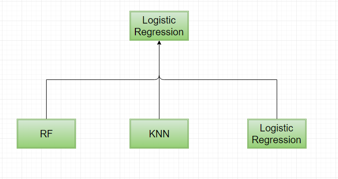
So far, we have used simple formulas at the top layer. Instead, we can use another machine learning model which is essentially what stacking is. We can use linear regression for making a linear formula for making the predictions in regression problem for mapping bottom layer model predictions to the outcome or logistic regression similarly in case of classification problem.
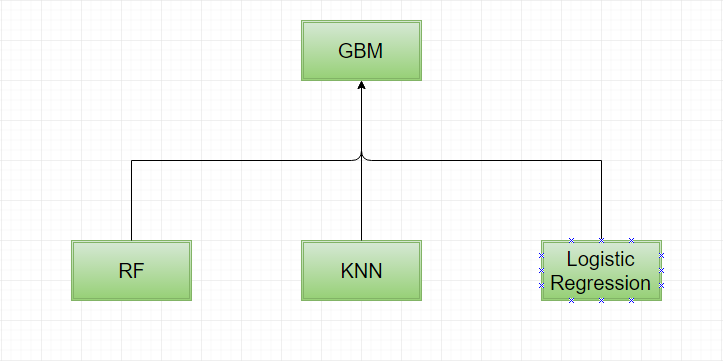
Moreover, we don’t need to restrict ourselves here, we can also use more complex models like GBM, neural nets to develop a non-linear mapping from the predictions of bottom layer models to the outcome.
On the same example let’s try applying logistic regression and GBM as top layer models. Remember, the following steps that we’ll take:
- Train the individual base layer models on training data.
- Predict using each base layer model for training data and test data.
- Now train the top layer model again on the predictions of the bottom layer models that has been made on the training data.
- Finally, predict using the top layer model with the predictions of bottom layer models that has been made for testing data.
One extremely important thing to note in step 2 is that you should always make out of bag predictions for the training data, otherwise the importance of the base layer models will only be a function of how well a base layer model can recall the training data.
Even, most of the steps have been already done previously, but I’ll walk you through the steps one by one again.
-
Step 1: Train the individual base layer models on training data
#Defining the training control
fitControl <- trainControl(
method = "cv",
number = 10,
savePredictions = 'final', # To save out of fold predictions for best parameter combinantions
classProbs = T # To save the class probabilities of the out of fold predictions
)

#Defining the predictors and outcome
predictors<-c("Credit_History", "LoanAmount", "Loan_Amount_Term", "ApplicantIncome",
"CoapplicantIncome")
outcomeName<-'Loan_Status'

#Training the random forest model
model_rf<-train(trainSet[,predictors],trainSet[,outcomeName],method='rf',trControl=fitControl,tuneLength=3

#Training the knn model
model_knn<-train(trainSet[,predictors],trainSet[,outcomeName],method='knn',trControl=fitControl,tuneLength=3)

#Training the logistic regression model
model_lr<-train(trainSet[,predictors],trainSet[,outcomeName],method='glm',trControl=fitControl,tuneLength=3)
-
Step 2: Predict using each base layer model for training data and test data
#Predicting the out of fold prediction probabilities for training data
trainSet$OOF_pred_rf<-model_rf$pred$Y[order(model_rf$pred$rowIndex)]
trainSet$OOF_pred_knn<-model_knn$pred$Y[order(model_knn$pred$rowIndex)]
trainSet$OOF_pred_lr<-model_lr$pred$Y[order(model_lr$pred$rowIndex)]

#Predicting probabilities for the test data
testSet$OOF_pred_rf<-predict(model_rf,testSet[predictors],type='prob')$Y
testSet$OOF_pred_knn<-predict(model_knn,testSet[predictors],type='prob')$Y
testSet$OOF_pred_lr<-predict(model_lr,testSet[predictors],type='prob')$Y
-
Step 3: Now train the top layer model again on the predictions of the bottom layer models that has been made on the training data
First, let’s start with the GBM model as the top layer model.
#Predictors for top layer models
predictors_top<-c('OOF_pred_rf','OOF_pred_knn','OOF_pred_lr')

#GBM as top layer model
model_gbm<-
train(trainSet[,predictors_top],trainSet[,outcomeName],method='gbm',trControl=fitControl,tuneLength=3)
Similarly, we can create an ensemble with logistic regression as the top layer model as well.
#Logistic regression as top layer model
model_glm<-
train(trainSet[,predictors_top],trainSet[,outcomeName],method='glm',trControl=fitControl,tuneLength=3)
-
Step 4: Finally, predict using the top layer model with the predictions of bottom layer models that has been made for testing data
#predict using GBM top layer model
testSet$gbm_stacked<-predict(model_gbm,testSet[,predictors_top])

#predict using logictic regression top layer model
testSet$glm_stacked<-predict(model_glm,testSet[,predictors_top])
Great! You made your first ensemble.
Note it’s really important to choose the models for the ensemble wisely to get the best out of the ensemble. The two thumb rules that we discussed will greatly help you in that.
5. Additional resources
By now, you might have developed an in-depth conceptual as well as practical knowledge of ensembling. I would like to encourage you to practice this on machine learning hackathons on Analytics Vidhya, which you can find here.
You’ll probably find this article on top five questions related to ensembling helpful.
Also, if you missed out on the skilltest on ensembling, you can check your understanding of ensembling concepts here.
End Notes
Ensembling is a very popular and effective technique that is very frequently used by data scientists for beating the accuracy benchmark of even the best of individual algorithms. More often than not it’s the winning recipe in hackathons. The more you’ll use ensembling, the more you’ll admire its beauty.
Did you enjoy reading this article? Do share your views in the comment section below. If you have any doubts / questions feel free to drop them in the comments below.


