Introduction
News media has become a channel to pass on the information of what’s happening in the world to the people living. Often people perceive whatever conveyed in the news to be true. There were circumstances where even the news channels acknowledged that their news is not true as they wrote. But some news has a significant impact not only on the people or government but also on the economy. One news can shift the curves up and down depending on the emotions of people and political situation.
It is important to identify the fake news from the real true news. The problem has been taken over and resolved with the help of Natural Language Processing tools which help us identify fake or true news based on historical data. The news is now in safe hands!
Problem statement
The authenticity of Information has become a longstanding issue affecting businesses and society, both for printed and digital media. On social networks, the reach and effects of information spread occur at such a fast pace and so amplified that distorted, inaccurate, or false information acquires a tremendous potential to cause real-world impacts, within minutes, for millions of users. Recently, several public concerns about this problem and some approaches to mitigate the problem were expressed.
The sensationalism of not-so-accurate eye-catching and intriguing headlines aimed at retaining the attention of audiences to sell information has persisted all throughout the history of all kinds of information broadcast. On social networking websites, the reach and effects of information spread are however significantly amplified and occur at such a fast pace, that distorted, inaccurate, or false information acquires a tremendous potential to cause real impacts, within minutes, for millions of users.
Objective
- Our sole objective is to classify the news from the dataset as fake or true news.
- Extensive EDA of news
- Selecting and building a powerful model for classification
Import Libraries
Let’s import all necessary libraries for the analysis and along with it let’s bring down our dataset
#Basic libraries
import pandas as pd
import numpy as np

#Visualization libraries
import matplotlib.pyplot as plt
from matplotlib import rcParams
import seaborn as sns
from textblob import TextBlob
from plotly import tools
import plotly.graph_objs as go
from plotly.offline import iplot
%matplotlib inline
plt.rcParams['figure.figsize'] = [10, 5]
import cufflinks as cf
cf.go_offline()
cf.set_config_file(offline=False, world_readable=True)

#NLTK libraries
import nltk
import re
import string
from nltk.corpus import stopwords
from wordcloud import WordCloud,STOPWORDS
from nltk.stem.porter import PorterStemmer
from sklearn.feature_extraction.text import TfidfVectorizer
from sklearn.feature_extraction.text import CountVectorizer
# Machine Learning libraries
import sklearn
from sklearn.model_selection import GridSearchCV
from sklearn.linear_model import LogisticRegression
from sklearn.tree import DecisionTreeClassifier
from sklearn.naive_bayes import MultinomialNB
from sklearn.neighbors import KNeighborsClassifier
from sklearn.model_selection import train_test_split


#Metrics libraries
from sklearn import metrics
from sklearn.metrics import classification_report
from sklearn.model_selection import cross_val_score
from sklearn.metrics import roc_auc_score
from sklearn.metrics import roc_curve
from sklearn.metrics import confusion_matrix
from sklearn.metrics import accuracy_score

#Miscellanous libraries
from collections import Counter

#Ignore warnings
import warnings
warnings.filterwarnings('ignore')

#Deep learning libraries
from tensorflow.keras.layers import Embedding
from tensorflow.keras.preprocessing.sequence import pad_sequences
from tensorflow.keras.models import Sequential
from tensorflow.keras.preprocessing.text import one_hot
from tensorflow.keras.layers import LSTM
from tensorflow.keras.layers import Bidirectional
from tensorflow.keras.layers import Dense
from tensorflow.keras.layers import Dropout
Importing the dataset
Let’s welcome our dataset and see what’s inside the box
#reading the fake and true datasets
fake_news = pd.read_csv('../input/fake-and-real-news-dataset/Fake.csv')
true_news = pd.read_csv('../input/fake-and-real-news-dataset/True.csv')

# print shape of fake dataset with rows and columns and information
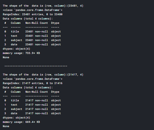
print ("The shape of the  data is (row, column):"+ str(fake_news.shape))
print (fake_news.info())
print("\n --------------------------------------- \n")

# print shape of true dataset with rows and columns and information
print ("The shape of the  data is (row, column):"+ str(true_news.shape))
print (true_news.info())
Dataset Details
This metadata has 2 CSV files where one dataset contains fake news and the other contains true/real news and has nearly 23481 fake news and 21417 true news
Description of columns in the file:
- title- contains news headlines
- text- contains news content/article
- subject- the type of news
- date- the date the news was published
Preprocessing and Cleaning
We have to perform certain pre-processing steps before performing EDA and giving the data to the model. Let’s begin with creating the output column
Creating the target column
Let’s create the target column for both fake and true news. Here we are gonna denote the target value as ‘0’ in case of fake news and ‘1’ in case of true news
#Target variable for fake news
fake_news['output']=0

#Target variable for true news
true_news['output']=1
Concatenating title and text of news
News has to be classified based on the tile and text jointly. Treating the title and content of news separately doesn’t reap any benefit. So, let’s concatenate both the columns in both datasets
#Concatenating and dropping for fake news
fake_news['news']=fake_news['title']+fake_news['text']
fake_news=fake_news.drop(['title', 'text'], axis=1)

#Concatenating and dropping for true news
true_news['news']=true_news['title']+true_news['text']
true_news=true_news.drop(['title', 'text'], axis=1)

#Rearranging the columns
fake_news = fake_news[['subject', 'date', 'news','output']]
true_news = true_news[['subject', 'date', 'news','output']]
Converting the date columns to datetime format
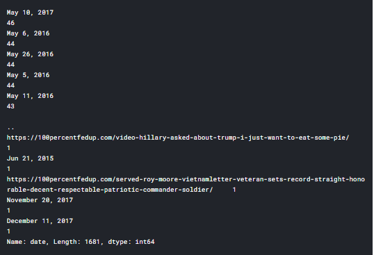
We can use pd.datetime to convert our date columns to date format we desire. But there was a problem, especially in fake_news date column. Let’s check the value_counts() to see what lies inside
fake_news['date'].value_counts()
If you notice, we had links and news headlines inside the date column which can give us trouble when converting to datetime format. So let’s remove those records from the column.
#Removing links and the headline from the date column
fake_news=fake_news[~fake_news.date.str.contains("http")]
fake_news=fake_news[~fake_news.date.str.contains("HOST")]

'''You can also execute the below code to get the result
which allows only string which has the months and rest are filtered'''
#fake_news=fake_news[fake_news.date.str.contains("Jan|Feb|Mar|Apr|May|Jun|Jul|Aug|Sep|Oct|Nov|Dec")]
Only the fake news dataset had an issue with the date column. Now let’s proceed with converting the date column to datetime format
#Converting the date to datetime format
fake_news['date'] = pd.to_datetime(fake_news['date'])
true_news['date'] = pd.to_datetime(true_news['date'])
Appending two datasets
When we are providing a dataset for the model, we have to provide it as a single file. So it’s better to append both true and fake news data and preprocess it further and perform EDA
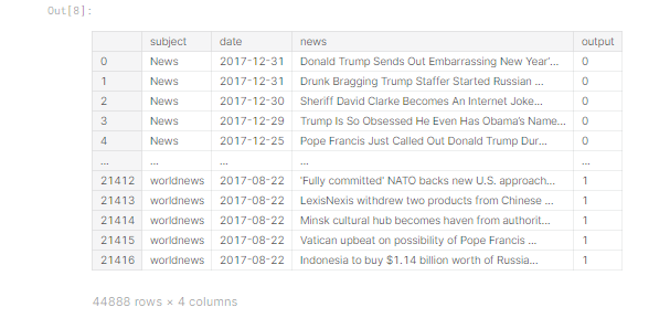
frames = [fake_news, true_news]
news_dataset = pd.concat(frames)
news_dataset
Text Processing
This is an important phase for any text analysis application. There will be much un-useful content in the news which can be an obstacle when feeding to a machine learning model. Unless we remove them the machine learning model doesn’t work efficiently. Let’s go step by step.
News-Punctuation Cleaning
Let’s begin our text processing by removing the punctuations
#Creating a copy
clean_news=news_dataset.copy()def review_cleaning(text):
    '''Make text lowercase, remove text in square brackets,remove links,remove punctuation
    and remove words containing numbers.'''
    text = str(text).lower()
    text = re.sub('\[.*?\]', '', text)
    text = re.sub('https?://\S+|www\.\S+', '', text)
    text = re.sub('<.*?>+', '', text)
    text = re.sub('[%s]' % re.escape(string.punctuation), '', text)
    text = re.sub('\n', '', text)
    text = re.sub('\w*\d\w*', '', text)
    return textclean_news['news']=clean_news['news'].apply(lambda x:review_cleaning(x))
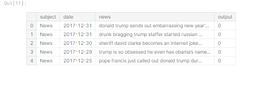
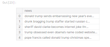
clean_news.head()
We have removed all punctuation in our news column.
News-Stop words
A stop word is a commonly used word (such as “the”, “a”, “an”, “in”) that a search engine has been programmed to ignore, both when indexing entries for searching and when retrieving them as the result of a search query. We would not want these words to take up space in our database, or taking up the valuable processing time. For this, we can remove them easily, by storing a list of words that you consider to stop words. NLTK(Natural Language Toolkit) in python has a list of stopwords stored in 16 different languages. Source: Geeks for Geeks
For our project, we are considering the English stop words and removing those words
stop = stopwords.words('english')
clean_news['news'] = clean_news['news'].apply(lambda x: ' '.join([word for word in x.split() if word not in (stop)]))
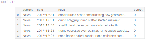
clean_news.head()
We have removed all the stop words in the review column.
Story Generation and Visualization from news
In this section, we will complete do exploratory data analysis on news such as ngram analysis and understand which are all the words, context which is most likely found in fake news.
Important note: Please check my kaggle notebook to find the coding part of the plots
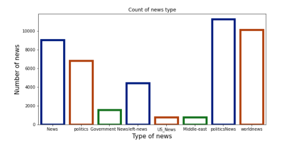
Count of the news subject
Let’s start by looking at the count of news types in our dataset
Insights:
- Our dataset has more political news than any other news followed by world news
- We have some repeated class names which express the same meaning such as news, politics, government news, etc which is similar to the alternative
Count of news subject based on true or fake
Let’s look at the count based on the fake/true outcome.
Insights:
- Fake news is all over the category except politics and world news
- The true news is present only in politics and world news and the count is high
- THIS IS A HIGHLY BIASED DATASET and we can expect higher accuracy which doesn’t signify it is a good model considering the poor quality of the dataset.
Count of fake news and true news
Let’s check the count of fake and true news and confirm whether our data is balanced or not
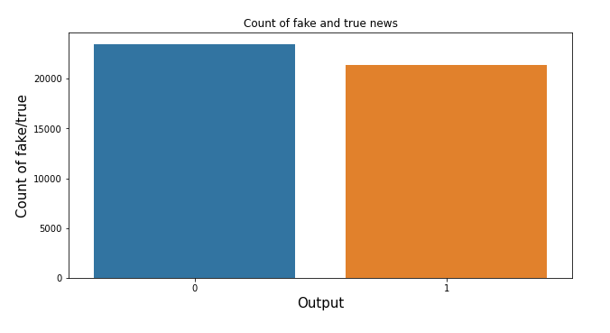
Insights:
- We have a pretty much-balanced data
- But the count of fake news is higher than the true news but not to a greater extent
Deriving new features from the news
Let’s extract more features from the news feature such as
- Polarity: The measure which signifies the sentiment of the news
- Review length: Length of the news(number of letters and spaces)
- Word Count: Number of words in the news
Insights:
- Most of the polarity is neutral, neither it shows some bad news nor much happy news
- The word count is between 0–1000 and the length of the news are between 0–5000 and a few near 10000 words which could be an article
N-gram analysis
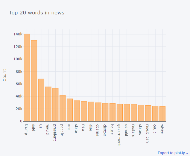
Top 20 words in News
Let’s look at the top 20 words from the news which could give us a brief idea of what news are popular in our dataset
Insights:
- All the top 20 news are about the US government
- Especially it’s about Trump and the US followed by Obama
- We can understand that the news is from Reuters.
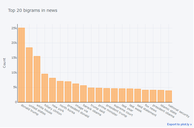
Top 2 words in the news
Now let’s expand our search to the top 2 words from the news
Insights:
- As feared, I think the model will be biased in its results considering the amount of trump news
- We can see the North Korea news as well, I think it will be about the dispute between the US and NK
- There is also some news from fox news as well
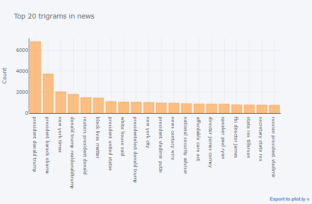
Top 3 words in the news
Now let’s expand our search to the top 3 words from the news
Insights:
- There is important news that ruled the US media-’Black lives matter’ post the demise of Floyd. We can see that news has been covered in our data. There was a lot of fake news revolved around death.
- The rest of the news is about US politics
WordCloud of Fake and True News
Let’s look at the word cloud for both fake and true news
Fake news
True news
Insights:
- True news doesn’t involve much trump instead on Republican Party and Russia
- There are news about Budget, military which comes under government news
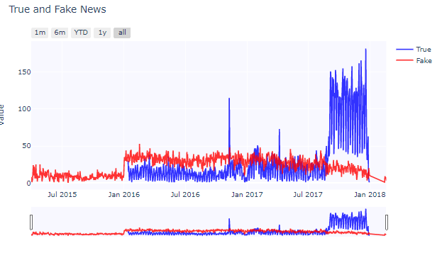
Time series analysis- Fake/True news
Let’s look at the timeline of true and fake news that were circulated in the media.
Insights:
- True news got their dominance since Aug 2017. As they are seen at a very higher rate. That is a good sign
- There are few outliers in true news where it was higher than the fake news(Nov 9, 2016, and Apr 7, 2017)
- Our dataset has more fake news than the true one as we can see that we don’t have true news data for the whole of 2015, So the fake news classification will be pretty accurate than the true news getting classified
Stemming the reviews
Stemming is a method of deriving root words from the inflected word. Here we extract the reviews and convert the words in reviews to their root word. for example,
- Going->go
- Finally->fina
If you notice, the root words don’t need to carry semantic meaning. There is another technique knows as Lemmatization where it converts the words into root words that have semantic meaning. Since it takes time. I’m using stemming
#Extracting 'reviews' for processing
news_features=clean_news.copy()
news_features=news_features[['news']].reset_index(drop=True)
news_features.head()
stop_words = set(stopwords.words("english"))
#Performing stemming on the review dataframe
ps = PorterStemmer()

#splitting and adding the stemmed words except stopwords
corpus = []
for i in range(0, len(news_features)):
    news = re.sub('[^a-zA-Z]', ' ', news_features['news'][i])
    news= news.lower()
    news = news.split()
    news = [ps.stem(word) for word in news if not word in stop_words]
    news = ' '.join(news)
    corpus.append(news)#Getting the target variable
y=clean_news['output']
Deep learning-LSTM
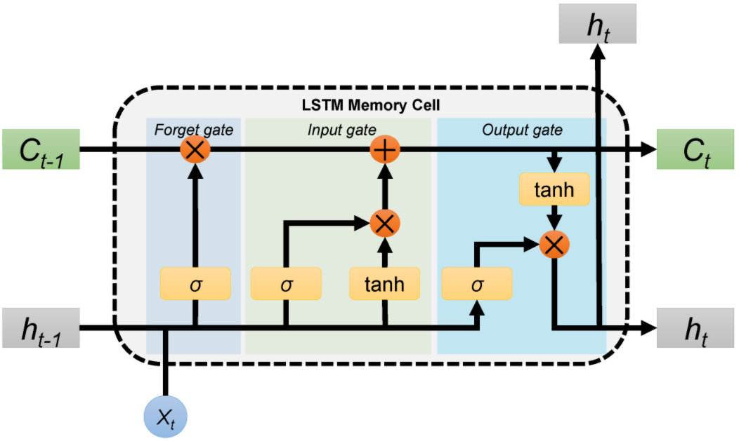
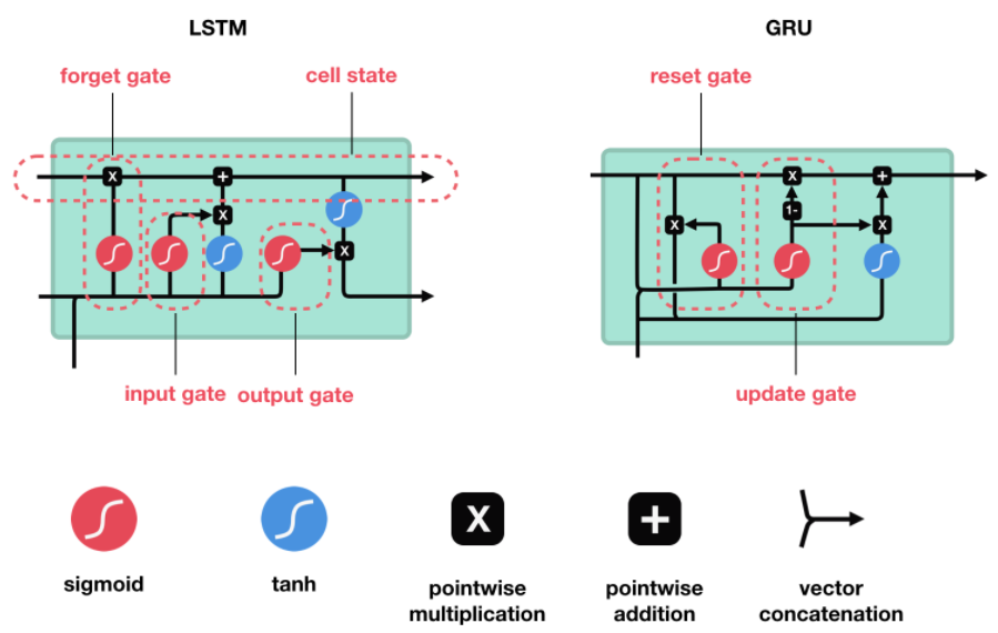
Please refer to this amazing article to know more about LSTM
Here in this part, we use a neural network to predict whether the given news is fake or not.
We aren’t gonna use a normal neural network like ANN to classify but LSTM(long short-term memory) which helps in containing sequence information. Long Short-Term Memory (LSTM) networks are a type of recurrent neural network capable of learning order dependence in sequence prediction problems. This is a behavior required in complex problem domains like machine translation, speech recognition, and more.
One hot for Embedding layers
Before jumping into creating a layer let’s take some vocabulary size. There might be a question of why vocabulary size? it is because we will be one hot encoding the sentences in the corpus for embedding layers. While one-hot encoding the words in sentences will take the index from the vocabulary size. Let’s fix the vocabulary size to 10000
#Setting up vocabulary size
voc_size=10000

#One hot encoding
onehot_repr=[one_hot(words,voc_size)for words in corpus]
Padding embedded documents
All the neural networks require to have inputs that have the same shape and size. However, when we pre-process and use the texts as inputs for our LSTM model, not all the sentences have the same length. In other words, naturally, some of the sentences are longer or shorter. We need to have the inputs of the same size, this is where the padding is necessary. Here we take the common length as 5000 and perform padding using pad_sequence() function. Also, we are going to ‘pre’ pad so that zeros are added before the sentences to make the sentence of equal length
#Setting sentence length
sent_length=5000

#Padding the sentences
embedded_docs=pad_sequences(onehot_repr,padding='pre',maxlen=sent_length)
print(embedded_docs)
We can see all the sentences are of equal length with the addition of zeros in front of the sentences and making all the sentences of length 5000.
LSTM Model
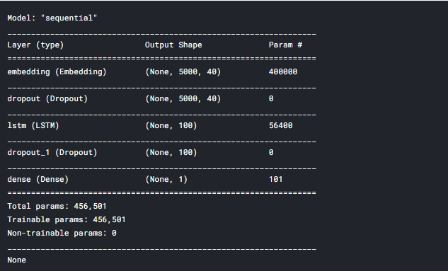
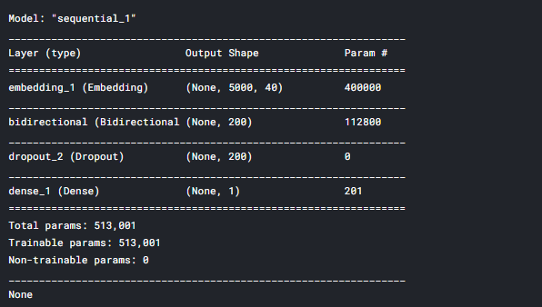
At first, we are going to develop the base model and compile it. The first layer will be the embedding layer which has the input of vocabulary size, vector features, and sentence length. Later we add a 30% dropout layer to prevent overfitting and the LSTM layer which has 100 neurons in the layer. In the final layer, we use the sigmoid activation function. Later we compile the model using adam optimizer and binary cross-entropy as loss function since we have only two outputs.
To understand how LSTM works please check this link. To give a small overview of how LSTM works, it remembers only the important sequence of words and forgets the insignificant words which don’t add value to the prediction.
#Creating the lstm model
embedding_vector_features=40
model=Sequential()
model.add(Embedding(voc_size,embedding_vector_features,input_length=sent_length))
model.add(Dropout(0.3))
model.add(LSTM(100)) #Adding 100 lstm neurons in the layer
model.add(Dropout(0.3))
model.add(Dense(1,activation='sigmoid'))

#Compiling the model
model.compile(loss='binary_crossentropy',optimizer='adam',metrics=['accuracy'])
print(model.summary())
Fitting the LSTM Model
Before fitting to the model, let’s consider the padded embedded object as X and y as y itself and convert them into an array.
# Converting the X and y as array
X_final=np.array(embedded_docs)
y_final=np.array(y)

#Check shape of X and y final
X_final.shape,y_final.shape
Let’s split our new X and y variable into train and test and proceed with fitting the model to the data. We have considered 10 epochs and 64 as batch size. It can be varied to get better results.
# Train test split of the X and y final
X_train, X_test, y_train, y_test = train_test_split(X_final, y_final, test_size=0.33, random_state=42)

# Fitting with 10 epochs and 64 batch size
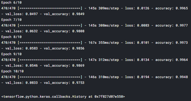
model.fit(X_train,y_train,validation_data=(X_test,y_test),epochs=10,batch_size=64)
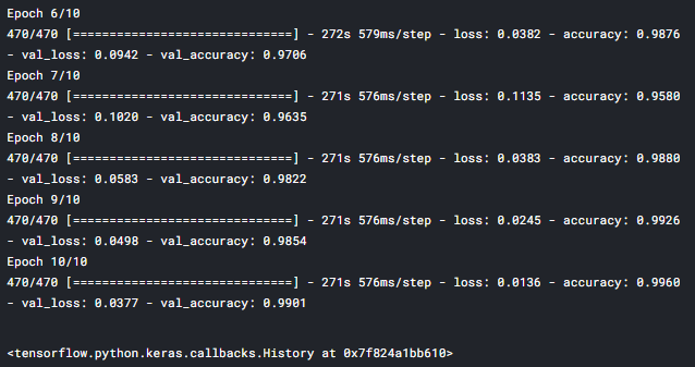
Last 4 epochs
Evaluation of model
Now, let’s predict the output for our test data and evaluate the predicted values with y_test. Check my kaggle notebook to find the function for the confusion matrix
# Predicting from test data
y_pred=model.predict_classes(X_test)

#Creating confusion matrix
#confusion_matrix(y_test,y_pred)
cm = metrics.confusion_matrix(y_test, y_pred)
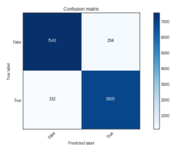
plot_confusion_matrix(cm,classes=['Fake','True'])
#Checking for accuracy
accuracy_score(y_test,y_pred)
We have got an accuracy of 96%. That’s awesome!
# Creating classification report
print(classification_report(y_test,y_pred))
From the classification report, we can see the accuracy value is nearly around 96%. We have to concentrate on the precision score and it is 96% which is great.
Bidirectional LSTM
Bi-LSTM is an extension of normal LSTM with two independent RNN’s together. The normal LSTM is unidirectional where it cannot know the future words whereas in Bi-LSTM we can predict the future use of words as there is backward information passed on from the other RNN layer in reverse.
There is only one change made in the code compared to the LSTM, here we use Bidirectional() function and call LSTM inside.
# Creating bidirectional lstm model
embedding_vector_features=40
model1=Sequential()
model1.add(Embedding(voc_size,embedding_vector_features,input_length=sent_length))
model1.add(Bidirectional(LSTM(100))) # Bidirectional LSTM layer
model1.add(Dropout(0.3))
model1.add(Dense(1,activation='sigmoid'))
model1.compile(loss='binary_crossentropy',optimizer='adam',metrics=['accuracy'])
print(model1.summary())
Fitting and Evaluation of Model
Let’s now fit the bidirectional LSTM model to the data we have with the same parameters we had before
# Fitting the model
model1.fit(X_train,y_train,validation_data=(X_test,y_test),epochs=10,batch_size=64)
# Predicting from test dataset
y_pred1=model1.predict_classes(X_test)

#Confusion matrix
cm = metrics.confusion_matrix(y_test, y_pred1)
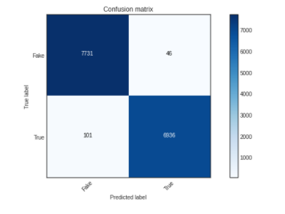
plot_confusion_matrix(cm,classes=['Fake','True'])
#Calculating Accuracy score
accuracy_score(y_test,y_pred1)
We have got an accuracy of 99%. That’s better than LSTM!
# Creating classification report
print(classification_report(y_test,y_pred1))
From the classification report, we can see the accuracy value is nearly around 99%. We have to concentrate on the precision score and it is 99%.
Conclusion
We have done mainstream work on processing the data and building the model. We could have indulged in changing the ngrams while vectorizing the text data. We took 2 words and vectorized them. You can check Shreta’s work on the same dataset where she got better results by considering both 1 and 2 words and also way better results with the help of LSTM and Bi-LSTM network. Let’s discuss the general insights from the dataset.
- Most of the fake news is surrounded by Election news and about Trump. Considering the US elections 2020. There are chances to spread fake news and the application of this technology will be heavily required.
- Fake news is currently rooted during this pandemic situation to play politics and to scare people and force them to buy goods
- Most of the news is from Reuters. We don’t know whether this news media is politically influenced. So we should always consider the source of news to find if the news is fake or true.
You can check Josué Nascimento’s work where he has explained why this dataset is more biased
You can also check out my other articles here.
Author
Ben Roshan













… [Trackback]
[…] Here you can find 98667 more Info to that Topic: geeksforgeeks.org/fake-news-classifier-on-us-election-news-lstm-wu/ […]