Decision Tree – A Step-by-Step Guide

Introduction to Decision Tree

Decision trees are a popular machine learning algorithm that can be used for both regression and classification tasks. They are easy to understand, interpret, and implement, making them an ideal choice for beginners in the field of machine learning. In this comprehensive guide, we will cover all aspects of the decision tree algorithm, including the working principles, different types of decision trees, the process of building decision trees, and how to evaluate and optimize decision trees. By the end of this article, you will have a complete understanding of decision trees and how they can be used to solve real-world problems. Please check the decision tree full course tutorial for FREE given below.

This article was published as a part of the Data Science Blogathon!

What is a Decision Tree?

A decision tree is a non-parametric supervised learning algorithm for classification and regression tasks. It has a hierarchical tree structure consisting of a root node, branches, internal nodes, and leaf nodes. Decision trees are used for classification and regression tasks, providing easy-to-understand models.

A decision tree is a hierarchical model used in decision support that depicts decisions and their potential outcomes, incorporating chance events, resource expenses, and utility. This algorithmic model utilizes conditional control statements and is non-parametric, supervised learning, useful for both classification and regression tasks. The tree structure is comprised of a root node, branches, internal nodes, and leaf nodes, forming a hierarchical, tree-like structure.

It is a tool that has applications spanning several different areas. Decision trees can be used for classification as well as regression problems. The name itself suggests that it uses a flowchart like a tree structure to show the predictions that result from a series of feature-based splits. It starts with a root node and ends with a decision made by leaves.

Decision Tree Terminologies

Before learning more about decision trees let’s get familiar with some of the terminologies:

• Root Node: The initial node at the beginning of a decision tree, where the entire population or dataset starts dividing based on various features or conditions.
• Decision Nodes: Nodes resulting from the splitting of root nodes are known as decision nodes. These nodes represent intermediate decisions or conditions within the tree.
• Leaf Nodes: Nodes where further splitting is not possible, often indicating the final classification or outcome. Leaf nodes are also referred to as terminal nodes.
• Sub-Tree: Similar to a subsection of a graph being called a sub-graph, a sub-section of a decision tree is referred to as a sub-tree. It represents a specific portion of the decision tree.
• Pruning: The process of removing or cutting down specific nodes in a decision tree to prevent overfitting and simplify the model.
• Branch / Sub-Tree: A subsection of the entire decision tree is referred to as a branch or sub-tree. It represents a specific path of decisions and outcomes within the tree.
• Parent and Child Node: In a decision tree, a node that is divided into sub-nodes is known as a parent node, and the sub-nodes emerging from it are referred to as child nodes. The parent node represents a decision or condition, while the child nodes represent the potential outcomes or further decisions based on that condition.

Example of Decision Tree

Let’s understand decision trees with the help of an example:

Decision trees are upside down which means the root is at the top and then this root is split into various several nodes. Decision trees are nothing but a bunch of if-else statements in layman terms. It checks if the condition is true and if it is then it goes to the next node attached to that decision.

In the below diagram the tree will first ask what is the weather? Is it sunny, cloudy, or rainy? If yes then it will go to the next feature which is humidity and wind. It will again check if there is a strong wind or weak, if it’s a weak wind and it’s rainy then the person may go and play.

Did you notice anything in the above flowchart? We see that if the weather is cloudy then we must go to play. Why didn’t it split more? Why did it stop there?

To answer this question, we need to know about few more concepts like entropy, information gain, and Gini index. But in simple terms, I can say here that the output for the training dataset is always yes for cloudy weather, since there is no disorderliness here we don’t need to split the node further.

The goal of machine learning is to decrease uncertainty or disorders from the dataset and for this, we use decision trees.

Now you must be thinking how do I know what should be the root node? what should be the decision node? when should I stop splitting? To decide this, there is a metric called “Entropy” which is the amount of uncertainty in the dataset.

How decision tree algorithms work?

Decision Tree algorithm works in simpler steps

1. Starting at the Root: The algorithm begins at the top, called the “root node,” representing the entire dataset.
2. Asking the Best Questions: It looks for the most important feature or question that splits the data into the most distinct groups. This is like asking a question at a fork in the tree.
3. Branching Out: Based on the answer to that question, it divides the data into smaller subsets, creating new branches. Each branch represents a possible route through the tree.
4. Repeating the Process: The algorithm continues asking questions and splitting the data at each branch until it reaches the final “leaf nodes,” representing the predicted outcomes or classifications.

Decision Tree Assumptions

Several assumptions are made to build effective models when creating decision trees. These assumptions help guide the tree’s construction and impact its performance. Here are some common assumptions and considerations when creating decision trees:

Binary Splits

Decision trees typically make binary splits, meaning each node divides the data into two subsets based on a single feature or condition. This assumes that each decision can be represented as a binary choice.

Recursive Partitioning

Decision trees use a recursive partitioning process, where each node is divided into child nodes, and this process continues until a stopping criterion is met. This assumes that data can be effectively subdivided into smaller, more manageable subsets.

Feature Independence

Decision trees often assume that the features used for splitting nodes are independent. In practice, feature independence may not hold, but decision trees can still perform well if features are correlated.

Homogeneity

Decision trees aim to create homogeneous subgroups in each node, meaning that the samples within a node are as similar as possible regarding the target variable. This assumption helps in achieving clear decision boundaries.

Top-Down Greedy Approach

Decision trees are constructed using a top-down, greedy approach, where each split is chosen to maximize information gain or minimize impurity at the current node. This may not always result in the globally optimal tree.

Categorical and Numerical Features

Decision trees can handle both categorical and numerical features. However, they may require different splitting strategies for each type.

Overfitting

Decision trees are prone to overfitting when they capture noise in the data. Pruning and setting appropriate stopping criteria are used to address this assumption.

Impurity Measures

Decision trees use impurity measures such as Gini impurity or entropy to evaluate how well a split separates classes. The choice of impurity measure can impact tree construction.

No Missing Values

Decision trees assume that there are no missing values in the dataset or that missing values have been appropriately handled through imputation or other methods.

Equal Importance of Features

Decision trees may assume equal importance for all features unless feature scaling or weighting is applied to emphasize certain features.

No Outliers

Decision trees are sensitive to outliers, and extreme values can influence their construction. Preprocessing or robust methods may be needed to handle outliers effectively.

Sensitivity to Sample Size

Small datasets may lead to overfitting, and large datasets may result in overly complex trees. The sample size and tree depth should be balanced.

Entropy

Entropy is nothing but the uncertainty in our dataset or measure of disorder. Let me try to explain this with the help of an example.

Suppose you have a group of friends who decides which movie they can watch together on Sunday. There are 2 choices for movies, one is “Lucy” and the second is “Titanic” and now everyone has to tell their choice. After everyone gives their answer we see that “Lucy” gets 4 votes and “Titanic” gets 5 votes. Which movie do we watch now? Isn’t it hard to choose 1 movie now because the votes for both the movies are somewhat equal.

This is exactly what we call disorderness, there is an equal number of votes for both the movies, and we can’t really decide which movie we should watch. It would have been much easier if the votes for “Lucy” were 8 and for “Titanic” it was 2. Here we could easily say that the majority of votes are for “Lucy” hence everyone will be watching this movie.

In a decision tree, the output is mostly “yes” or “no”

The formula for Entropy is shown below:

Here,

• p₊ is the probability of positive class
• p_– is the probability of negative class
• S is the subset of the training example

How do Decision Trees use Entropy?

Now we know what entropy is and what is its formula, Next, we need to know that how exactly does it work in this algorithm.

Entropy basically measures the impurity of a node. Impurity is the degree of randomness; it tells how random our data is. Apure sub-splitmeans that either you should be getting “yes”, or you should be getting “no”.

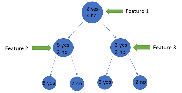
Supposea featurehas 8 “yes” and 4 “no” initially, after the first split the left node gets 5 ‘yes’ and 2 ‘no’whereas right node gets 3 ‘yes’ and 2 ‘no’.

We see here the split is not pure, why? Because we can still see some negative classes in both the nodes. In order to make a decision tree, we need to calculate the impurity of each split, and when the purity is 100%, we make it as a leaf node.

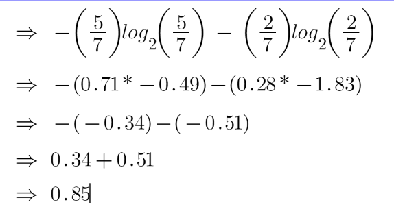
To check the impurity of feature 2 and feature 3 we will take the help for Entropy formula.

For feature 3,

We can clearly see from the tree itself that left node has low entropy or more purity than right node since left node has a greater number of “yes” and it is easy to decide here.

Always remember that the higher the Entropy, the lower will be the purity and the higher will be the impurity.

As mentioned earlier the goal of machine learning is to decrease the uncertainty or impurity in the dataset, here by using the entropy we are getting the impurity of a particular node, we don’t know if the parent entropy or the entropy of a particular node has decreased or not.

For this, we bring a new metric called “Information gain” which tells us how much the parent entropy has decreased after splitting it with some feature.

Information Gain

Information gain measures the reduction of uncertainty given some feature and it is also a deciding factor for which attribute should be selected as a decision node or root node.

It is just entropy of the full dataset – entropy of the dataset given some feature.

To understand this better let’s consider an example:Suppose our entire population has a total of 30 instances. The dataset is to predict whether the person will go to the gym or not. Let’s say 16 people go to the gym and 14 people don’t

Now we have two features to predict whether he/she will go to the gym or not.

• Feature 1 is “Energy” which takes two values “high” and “low”
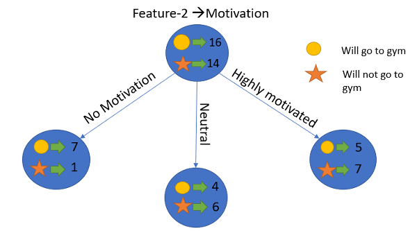
• Feature 2 is “Motivation” which takes 3 values “No motivation”, “Neutral” and “Highly motivated”.

Let’s see how our decision tree will be made using these 2 features. We’ll use information gain to decide which feature should be the root node and which feature should be placed after the split.

Let’s calculate the entropy

To see the weighted average of entropy of each node we will do as follows:

Now we have the value of E(Parent) and E(Parent|Energy), information gain will be:

Our parent entropy was near 0.99 and after looking at this value of information gain, we can say that the entropy of the dataset will decrease by 0.37 if we make “Energy” as our root node.

Similarly, we will do this with the other feature “Motivation” and calculate its information gain.

Let’s calculate the entropy here:

To see the weighted average of entropy of each node we will do as follows:

Now we have the value of E(Parent) and E(Parent|Motivation), information gain will be:

We now see that the “Energy” feature gives more reduction which is 0.37 than the “Motivation” feature. Hence we will select the feature which has the highest information gain and then split the node based on that feature.

In this example “Energy” will be our root node and we’ll do the same for sub-nodes. Here we can see that when the energy is “high” the entropy is low and hence we can say a person will definitely go to the gym if he has high energy, but what if the energy is low? We will again split the node based on the new feature which is “Motivation”.

When to Stop Splitting?

You must be asking this question to yourself that when do we stop growing our Decision tree? Usually, real-world datasets have a large number of features, which will result in a large number of splits, which in turn gives a huge tree. Such trees take time to build and can lead to overfitting. That means the tree will give very good accuracy on the training dataset but will give bad accuracy in test data.

There are many ways to tackle this problem through hyperparameter tuning. We can set the maximum depth of our decision tree using themax_depth parameter. The more the value of max_depth, the more complex your tree will be. The training error will off-course decrease if we increase the max_depth value but when our test data comes into the picture, we will get a very bad accuracy. Hence you need a value that will not overfit as well as underfit our data and for this, you can use GridSearchCV.

Another way is to set the minimum number of samples for each spilt. It is denoted by min_samples_split. Here we specify the minimum number of samples required to do a spilt. For example, we can use a minimum of 10 samples to reach a decision. That means if a node has less than 10 samples then using this parameter, we can stop the further splitting of this node and make it a leaf node.

There are more hyperparameters such as :

• min_samples_leaf – represents the minimum number of samples required to be in the leaf node. The more you increase the number, the more is the possibility of overfitting.
• max_features – it helps us decide what number of features to consider when looking for the best split.

To read more about these hyperparameters you can read ithere.

Pruning

Pruning is another method that can help us avoid overfitting. It helps in improving the performance of the Decision tree by cutting the nodes or sub-nodes which are not significant. Additionally, it removes the branches which have very low importance.

There are mainly 2 ways for pruning:

• Pre-pruning – we can stop growing the tree earlier, which means we can prune/remove/cut a node if it has low importance while growing the tree.
• Post-pruning – once our tree is built to its depth, we can start pruning the nodes based on their significance.

Conclusion

To summarize, in this article we learned about decision trees. On what basis the tree splits the nodes and how to can stop overfitting. why linear regression doesn’t work in the case of classification problems.To check out the full implementation of decision trees please refer to my Github repository. You can master all the Data Science topics with our Black Belt Plus Program with out 50+ projects and 20+ tools. Start your learning journey today!

Frequently Asked Questions

Anshul Saini

05 Jan 2024

I am an undergraduate student currently in my last year majoring in Statistics (Bachelors of Statistics) and have a strong interest in the field of data science, machine learning, and artificial intelligence. I enjoy diving into data to discover trends and other valuable insights about the data. I am constantly learning and motivated to try new things.