Introduction
Algorithmic trading is a widely adopted trading strategy that has revolutionized the way people trade stocks. More and more people are making money on the side by investing in stocks and automating their trading strategies. This tutorial will teach you how to build stock trading algorithms using primitive technical indicators like MACD, SMA, EMA, etc., and select the best strategies based on their actual performance/returns, completely using Python.
Learning Objectives
- Get to know what algorithmic trading is.
- Build simple stock trading algorithms in Python, using technical indicators to generate buy and sell signals.
- Learn to implement trading strategies and automate them in Python.
- Learn to compare and select the best trading strategy based on their average returns.
This article was published as a part of the Data Science Blogathon.
Disclaimer – This is not financial advice, and all work done in this project is for educational purposes only.
Table of Contents
What is Algorithmic Trading?
Algorithmic trading is a method of trading financial assets using automated computer programs to execute orders based on predefined rules and strategies. It involves the use of several trading strategies, including statistical arbitrage, trend following, and mean reversion to name a few.
There are many different types of algorithmic trading. One of them is high-frequency trading, which involves executing trades at high speeds with almost no latency to take advantage of small price movements. Another is news-based trading, which involves making trades based on news and other market events.
In this article, we will be using Python to do stock trading based on technical indicators and candlestick pattern detection.
How to Use Python Algorithms for Stock Trading Analysis?
We can analyze the stock market, figure out trends, develop trading strategies, and set up signals to automate stock trading – all using Python! The process of algorithmic trading using Python involves a few steps such as selecting the database, installing certain libraries, and historical data extraction. Let us now delve into each of these steps and learn to build simple stock trading algorithms.
Selecting the Dataset
There are thousands of publicly traded stocks and we can consider any set of stocks for building the algorithm. However, it is always a good option to consider similar kinds of stocks as their fundamentals and technicals will be comparable.
In this article, we will be considering the Nifty 50 stocks. Nifty 50 index consists of 50 of the top companies in India chosen based on various factors such as market capitalization, liquidity, sector representation, and financial performance. The index is also widely used as a benchmark to measure the performance of the Indian stock market and as a result, there is a lesser amount of risk involved while investing in these companies when compared to investing in small-cap or mid-cap companies. I will consider WIPRO for performing the analysis in this article. The analysis approach discussed in this article can be performed on any set of similar stocks by calling the functions for each stock in a for loop.
Installing the Required Libraries
We will use the default libraries like pandas, numpy, matplotlib along with yfinance and pandas_ta. The yfinance library will be used to extract the historical stock prices. The pandas_ta library will be used for implementing the SMA and the MACD indicator and building the trading algorithm. These modules can be directly installed using pip like any other Python library. Let’s import the modules after installing them.
!pip install yfinance
!pip install pandas-ta
import yfinance as yf
import pandas as pd
import pandas_ta as ta
import numpy as np
from datetime import datetime as dt
import matplotlib.pyplot as plt
from datetime import timedelta as delta
import numpy as np
import os
import seaborn as sbNow that we have installed and imported all the required libraries, let’s get our hands dirty and start building the strategies.
Extracting the Historical Stock Prices Using yfinance
We will use the “download()” function from the yfinance module to extract the historical price of a stock, which accepts the stock’s picker, start date, and end date. For the sake of simplicity, we will take “2000-01-01” as the start date and the current date as the end date. We will write a simple function that extracts the historical stock prices and returns it as a data frame for processing further while saving it as a CSV file on our disk.
def get_stock_info(stock, save_to_disk=False):
    start_date = '2000-01-01'
    end_date = (dt.now() + delta(1)).strftime('%Y-%m-%d')
    df = yf.download(f"{stock}.NS", period='1d', start=start_date, end=end_date, progress=False)
    if(save_to_disk == True):
        path = './csv'
        try: os.mkdir(path)
        except OSError as error: pass
        df.to_csv(f'{path}/{stock}.csv')

    return df

df = get_stock_info('WIPRO', save_to_disk = True)
Building Stock Trading Algorithms Using Technical Indicators
There are numerous indicators available for performing stock trading but we will be using one of the two simplest yet extremely popular indicators namely, SMA and MACD. SMA stands for Simple Moving Average while MACD stands for Moving Average Convergence Divergence. In case you are not familiar with these terms, you can learn more about them in this article. In short, we will try to find the SMA crossover and MACD crossover as trade signals and try to find the best combination of the lot for maximized returns.
For the SMA crossover, we will take the 10-day, 30-day, 50-day, and 200-day moving averages into account. For the MACD crossover, we will take the 12-day, 26-day, and 9-day exponential moving averages into account. Let’s calculate these values using the pandas_ta library.
For calculating the SMA, we will use the “sma()” function by passing the adjusted close price of the stock along with the number of days. For calculating the MACD, we will use the “macd()” function by passing the adjusted close price of the stock and setting the fast, slow, and signal parameters as 12, 26, and 9 respectively. The SMA and MACD values don’t make a lot of sense as such. So, let’s encode them to understand if there are any crossovers.
In the case of SMA, we will take 3 conditions:
- The 10-day SMA should be above the 30-day SMA.
- The 10-day and 30-day SMA should be above the 50-day SMA.
- The 10-day, 30-day, and 50-day should be above the 200-day SMA.
In the case of MACD, we will have 2 conditions:
- The MACD should be above the MACD signal.
- The MACD should be greater than 0.
The Python code given below creates a function to implement the conditions mentioned above.
def add_signal_indicators(df):
    df['SMA_10'] = ta.sma(df['Adj Close'],length=10)
    df['SMA_30'] = ta.sma(df['Adj Close'],length=30)
    df['SMA_50'] = ta.sma(df['Adj Close'],length=50)
    df['SMA_200'] = ta.sma(df['Adj Close'],length=200)

    macd = ta.macd(df['Adj Close'], fast=12, slow=26, signal=9)
    df['MACD'] = macd['MACD_12_26_9']
    df['MACD_signal'] = macd['MACDs_12_26_9']
    df['MACD_hist'] = macd['MACDh_12_26_9']

    df['10_cross_30'] = np.where(df['SMA_10'] > df['SMA_30'], 1, 0)

    df['MACD_Signal_MACD'] = np.where(df['MACD_signal'] < df['MACD'], 1, 0)

    df['MACD_lim'] = np.where(df['MACD']>0, 1, 0)

    df['abv_50'] = np.where((df['SMA_30']>df['SMA_50'])
            &(df['SMA_10']>df['SMA_50']), 1, 0)

    df['abv_200'] = np.where((df['SMA_30']>df['SMA_200'])
            &(df['SMA_10']>df['SMA_200'])&(df['SMA_50']>df['SMA_200']), 1, 0)

    return df

df =  add_signal_indicators(df)
Now that we have all the signals added to our data, it is time to calculate the returns. The returns will be the most important aspect for selecting the best trading strategy amongst the lot. We will calculate the 5-day and 10-day returns of the stock. We will also label encode the returns as 0 and 1 with 0 indicating negative returns and 1 indicating positive returns. Let’s go ahead and create the function implementing the same.
def calculate_returns(df):
    df['5D_returns'] = (df['Adj Close'].shift(-5)-df['Adj Close'])/df['Close']*100
    df['10D_returns'] = (df['Adj Close'].shift(-10)-df['Adj Close'])/df['Close']*100

    df['5D_positive'] = np.where(df['5D_returns']>0, 1, 0)
    df['10D_positive'] = np.where(df['10D_returns']>0, 1, 0)

    return df.dropna()


df = calculate_returns(df)
Understanding the Performance of the Signals
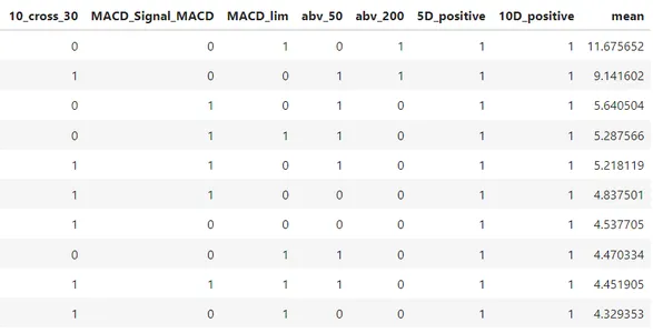
We can take all the conditions mentioned above and perform a simple aggregate to calculate the average and the median returns we can expect while trading based on these signals. We can also extract the minimum and the maximum returns each signal has generated in the past. This will not only give us a rough understanding of how good the signals are but also an idea of how much returns can be expected while trading using these signals. Let’s write a simple code to do the same using Python.
def get_eda_and_deepdive(df):
    eda = df.dropna().groupby(['10_cross_30', 'MACD_Signal_MACD',
    'MACD_lim', 'abv_50', 'abv_200'])[['5D_returns', '10D_returns']]\
    .agg(['count', 'mean','median', 'min', 'max'])

    deepdive = df.dropna().groupby(['10_cross_30', 'MACD_Signal_MACD',
     'MACD_lim', 'abv_50', 'abv_200','5D_positive', '10D_positive'])[['5D_returns', '10D_returns']]\
    .agg(['count', 'mean','median', 'min', 'max'])

    return eda, deepdive


eda, deepdive = get_eda_and_deepdive(df)
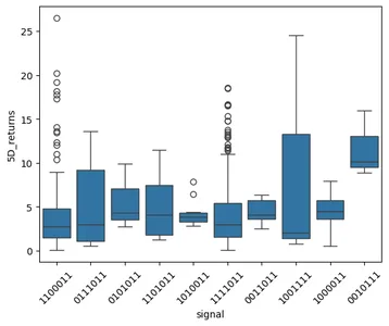
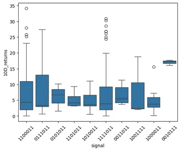
Let’s visualize the box whiskers plot for the top 10 signal combinations sorted based on the 5-day and the 10-day returns.
x = df.copy()

def _fun(x):
    code = ''
    for i in x.keys(): code += str(x[i])
    return code

x['signal'] = x[['10_cross_30', 'MACD_Signal_MACD', 'MACD_lim', 'abv_50', 'abv_200',
                     '5D_positive', '10D_positive']].apply(_fun, axis=1)

x = x.dropna()

lim = x.groupby(['10_cross_30', 'MACD_Signal_MACD', 'MACD_lim',
'abv_50', 'abv_200', '5D_positive', '10D_positive'])['5D_returns'].agg(['mean']).reset_index()
lim = lim.sort_values(by='mean', ascending=False).head(10)

x = x.merge(lim, on=['10_cross_30', 'MACD_Signal_MACD', 'MACD_lim',
 'abv_50', 'abv_200', '5D_positive', '10D_positive'], how='inner')
ax = sb.boxplot(x='signal', y='5D_returns', data=x)
ax.set_xticklabels(ax.get_xticklabels(), rotation=45)
plt.show()
ax = sb.boxplot(x='signal', y='10D_returns', data=x)
ax.set_xticklabels(ax.get_xticklabels(), rotation=45)
plt.show()
Taking only the 5-day and 10-day returns for selecting the best signals is not the best approach because we will never know how many times the signal has given positive returns against negative returns. This approach could be taken into account while selecting the best strategies, which could potentially improve the performance of the strategies. I will not take this approach to keep this article simple and beginner-friendly.
Conclusion
The concept of algorithmic trading can be extremely tempting for many as it can be very lucrative but at the same time, it tends to be an extremely complex and tedious task to build stock trading algorithms from scratch. It is very crucial to understand the fact that all algorithms can fail, which could potentially lead to huge financial losses when deployed to a live trading environment. The aim of this article was to explore how simple trading algorithms can be built and validated using Python. To proceed further in this project, you may consider other technical indicators and candlestick patterns, and use them interchangeably to build more complex algorithms and strategies.
Key Takeaways
- In this article, we learned to extract historical stock prices using yfinance.
- We learned to calculate MACD and SMA values based on the stock price and build Python algorithms to create signals/strategies using these values.
- We also learned to calculate and visualize the 5-day and 10-day returns of the strategies on the stock.
Note: This is not financial advice, and all work done in this project is for educational purposes only. That’s it for this article. Hope you enjoyed reading this article and learned something new. Thanks for reading and happy learning!
Frequently Asked Questions
Ans. No, all stock trading strategies are bound to fail and can lead to capital loss. The strategies used in this article are for educational purposes only. Do not use them to make financial investments.
Ans. Yes, these signals can be considered feature-engineered variables and can be used for performing machine learning or deep learning.
Ans. It is important to select similar stocks as their fundamentals and other parameters like alpha/beta will be comparable. The alpha and beta values of a large-cap company and a small-cap company might be in different ranges. Hence, it might not be right to randomly mix them while performing this analysis.
Ans. There are hundreds of indicators available and widely used for trading like RSI, MACD, and SMA. There are numerous technical candlestick indicators available as well like HARAMICROSS, MORNINGSTAR, and HAMMER that can help generate the signals.
Ans. This analysis can be performed for commodities with vast historical data. But in the case of cryptocurrencies, it depends on how much historical data is truly available. The analysis might fail or give a wrong conclusion if the signals occur a very times in the entire historical data.
The media shown in this article is not owned by Analytics Vidhya and is used at the Author’s discretion.

