Winners solutions and approach: Xtreme ML Hack, AV DataFest 2017

Introduction

Analytics Vidhya just completed 4 years and we had to make sure we mark this event in style! We did that by creating our most unique hackathon – Xtreme ML Hack as part of DataFest 2017. We were looking for an exciting real life problem and would want to thanks our sponsor – Aigues de Barcelona for providing us with an opportunity to host this wonderful competition.

Xtreme ML Hack started on 20 April 2017 and went on for 4 days. We saw more than 2400 participants from across the globe. There were multiple things which were unique for this competition. This was the first time we were working for a Spainish company. This was also an unique hackathon because the participants were allowed to use any available open data. Also, this was the fist time we were working with an utility company.

I think this was probably the most challenging hackathon we have released till now – this is as close as you can get to a real life project. Like always, the winners of the competition have generously shared their detailed approach and the codes they used in the competition.

If you missed out the fun, make sure you participate in the upcoming MiniHack – The QuickSolver.

About the Competition

The problem statement revolved around public-private company Aigües de Barcelona. It manages the integral cycle of water, from the uptake to the drinking process, transport and distribution, besides the sanitation and the purification of waste water for its return to the natural environment or its re-use. It offers service to about 3 million people in the municipalities of the metropolitan area of Barcelona. It also manages a customer service to ensure excellence in their services.

Customer Service is one of the top priorities of the company. They want to redesign the customer service using machine learning.

Problem Statement

To respond to their customers efficiently they want to predict the volume and typologies of contacts to the call center. They also want to forecast the number of contacts on daily basis. The task was to forecast the number of contacts & resolutions the company should open on daily basis.

• Contacts: A contact is defined whenever a customer initiates and gets in touch with the Company. The contact can happen through various channels including phone, mail, visit, fax etc.
• Resolutions: A Resolution is created every time a customer has placed a request with the company. This could be through a customer contact (as defined above) or otherwise (for example, when the company called the customer).

Winners

The winners used different approaches and rose up on the leaderboard. Below are the top 3 winners on the leaderboard:

Rank 1: Rohan Rao & Mark Landry

Rank 2: Sonny Laskar

Rank 3: Aanish Singla

Here are the final rankings of all the participants at the leaderboard.

All the Top 3 winners have shared their detailed approach & code from the competition. I am sure you are eager to know their secrets, go ahead.

Approach & code of all the winners

Aanish Singla, Rank 3

Here’s what Aanish shared with us.

Aanish says “I started out by building an understanding of how autonomous communities, provinces, municipalities and districts are related to each other in Spain. Then I looked at the data dictionary and what all was provided and what was expected, followed by exploratory data analysis.”

Key findings from analysis were

For Contacts:

1. Slightly increasing trend in recent years
2. August has a dip. December was the next lowest
3. 31st has a dip.
4. Volume by call input is highest (~75%), followed by visit and web (~10%)
5. Visits have increased in 2016
6. Web Inputs have increased significantly from 2015 onwards
7. Web Inputs are higher in Jan and then decrease for next 3-4 months and rise again in Sep-Nov
8. Contacts are low on weekends
9. Quarter also has an impact
10. Different contact types have different trends from past to recent

For Resolutions

1. Low volume on weekend pattern exists
2. Requests are increasing linearly by time but not so steeply for Barcelona, Badalona.
3. August has low resolutions
4. Technical claims, Non-Compliance have increased over time
5. Total resolutions have increased from 2014

I also figured out that there was a close correlation between new contracts, ended contracts and number of contacts. I had 2 choices.

1. To predict new contacts and ended contacts using time series and then predict contacts for them
2. Directly predict contacts using time series forecasting

I used the second approach.

Predicting contacts

I used top down approach as the there was only 1 level involved. I predicted the contacts at day level using Exponential smoothing state space model with Box-Cox transformation, ARMA errors, Trend and Seasonal components (tbats) using weekly, quarterly and yearly seasonality. To accommodate the trends at type level, I found the average contribution by type for 2016 and for all years (some types had different trends in recent years). Using separate contribution percentages by types and for weekdays and weekends, I split the overall forecast into detailed forecast.

Predicting Resolution

Resolutions had 2 levels (category and subject), hence top down approach was not suitable. Also, breaking the high-level forecast into 2 levels would be quite error prone so I selected hierarchical time series modeling for this. I used tbats() for each subject to account for multiple seasonality on the data. Most of the effort was in preparing data in the format accepted by hierarchical time series modeling function, hts(). I used only last 3 years of data (optimized after first submission) as that was having lesser missing values and avoided the spiked 2013 data. Combining of low level forecast with top level was done using LU decomposition algorithm.

Prediction from this resulted in some negative values, especially for the weekend. I replaced them with respective mean from 2016 weekend data.

On submission, I had a score of 104.6 but decided not to change the model too much as it was very generic.

Solution: Link to Code

Sonny Laskar, Rank 2

Here’s what Sonny shared with us.

He says “This was one of the best competitions till now on Analytics Vidhya. Moreover, the introduction of submission limits made it even more interesting. This competition was definitely not a good place to start from if you had just started learning ML. My first thought on looking at the problem made me think that it had to be solved as a time-series problem which later seemed to be wrong.”

Modeling Approach

It was a no-brainer to find that the only data in the Test Set were “future” dates. Did that look odd? Come to reality! The variable to predict was # of contacts/resolutions. After some initial analysis, I decided that this has to be treated as two different problems.

For the modeling purpose, I created day wise-medium wise-department wise aggregated # of contacts and resolutions from 2010 onwards (since we had data on contacts/resolutions only after 2010). For cross-validation, I decided to use the last four months. So my first model was built on few “Date” features and it scored 101.X which was a very good score on Day1.

The next thing that struck me was that holidays should have an impact on these contacts and resolutions. Hence I created a list of holidays in Spain since 2010. Just adding holidays to the above list improved the score to 93.X. I was feeling good but it didn’t last longer since I saw Mark jumping to 78.X.

Later, I decided to add “lag” features of # of contacts/resolutions from the past. After a few iterations, I decided to keep lag features of 75, 90 and 120 days. With this, the score improved to 64.X (ahead of Mark J). Rohan was around 114.X so I knew that he was either asleep or solving Soduku. This was on Saturday morning and I was unable to find any additional features that could help me move ahead. So I decided to take a break.  By evening, I noticed that Rohan had woken up and was also at around 78.X (That’s when I guess Mark and Rohan decided to team up).

On Sunday, I added a feature on number of days (percentile) elapsed since last holiday and that added few points. My final 10-bags XGboost ensemble scored 61.47081 on the public leaderboard which I selected for “final submission”. I had around 8 submissions left which I wish I could donate to few folks who were not aware that they could not mark their final submissions if they didn’t upload code L.

Huh!

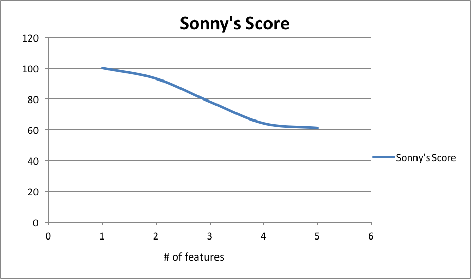
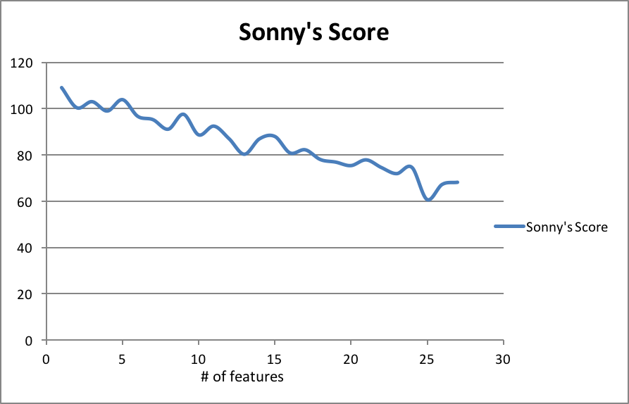
It might sound that the journey of adding features and improving scores was a very smooth line something like this.

But it was not. I tried many things which didn’t work.

Below are few approaches that I tried but didn’t seem to add value:

1. Using # of contracts added/ended data and using them as lagged featured
2. Predicting # of contracts added/ended (time-series and regression) and use them in model (While CV improved but the leaderboard dropped, may be because the predictions of contracts were themselves not correct)
3. Using contacts info for prediction of resolutions and vice-versa
4. Stage 2 meta modeling with predictions
5. Log and Square root transformation of contacts and resolutions
6. Time-series modeling approach instead of regression
7. And much more…

Overall, this was a different problem and really enjoyed solving it. Thanks to Mark and Rohan for a tough fight.

Rohan Rao & Mark Landry, Rank 1

Here’s what Mark & Rohan shared with us.

Mark Landry

Rohan Rao

I started exploring the data to get a sense of basic movement of values across the years. I decided to go with granularity and build a model for each type / category in Contacts and Resolution. I ultimately ended up plotting over 2000 graphs and summaries, which really helped identify various patterns.

After trying a bunch of features and models, I found historic averages out-performing all ML-based models. So, I decided to focus and tune the average values so as to capture seasonality and trend in the right way. In some ways, this was like a manually-customized time series model.

Main features

1. There were two highly seasonal components. Weekly and yearly. The following lag features: same week year and weekday in the previous year, previous/next week year and same weekday in the previous year, helped capture seasonality.

Besides these core features, other things that worked were:

1. Using 21st-Jan, 2016 to 15th-Mar, 2016 as the validation data. This helped in preventing overfitting to public LB.

2. Using estimates for holiday dates. Most holidays had 0 volume and highly noisy values. Aligning these correctly across the years helped.

3. My non-ML historic averages approach blended extremely well with Mark’s ML-model which didn’t use lag-features. Our simple ensemble gave a lift of almost 10 on RMSE.

4. Throw away all data prior to 2015, so as to focus only on the most recent trends.

Solution: Link to Code

End Notes

It was great fun interacting with these winners and to know their approach during the competition. Hopefully, you will be able to evaluate where you missed out.

Check out all the upcoming competitions here

Sunil Ray

02 May 2017

I am a Business Analytics and Intelligence professional with deep experience in the Indian Insurance industry. I have worked for various multi-national Insurance companies in last 7 years.