This article was published as a part of the Data Science Blogathon
Introduction
We all have made our resumes at some point in time. In a resume, we try to include important facts about ourselves like our education, work experience, skills, etc. Let us work on a resume dataset today.

The text we put in our resume speaks a lot about us. For example, our education, skills, work experience, and other random information about us are all present in a resume.
What is Text Analytics?
Text Analytics involves the use of unstructured text data, processing them into usable structured data. Text Analytics is an interesting application of Natural Language Processing. Text Analytics has various processes including cleaning of text, removing stopwords, word frequency calculation, and much more.
Text Analytics has gained much importance these days. As millions of people engage in online platforms and communicate with each other, a large amount of text data is generated. Text data can be blogs, social media posts, tweets, product reviews, surveys, forum discussions, and much more. Such huge amounts of data create huge text data for organizations to use. Most of the text data available are unstructured and scattered. Text analytics is used to gather and process this vast amount of information to gain insights.
Text Analytics serves as the foundation of many advanced NLP tasks like Classification, Categorization, Sentiment Analysis, and much more. Text Analytics is used to understand patterns and trends in text data. Keywords, topics, and important features of Text are found using Text Analytics.
Some Important uses of Text Analytics:
Some of the most important and interesting uses of Text Analytics is-
1. Scientific Discovery
2. Records Management and Analytics
3. Social Media Monitoring
4. Resume Filtering
5. Competitive Intelligence
There are many more interesting aspects of Text Analytics, now let us proceed with our resume dataset. The dataset contains text from various resume types and can be used to understand what people mainly use in resumes.
Resume Text Analytics is often used by recruiters to understand the profile of applicants and filter applications. Recruiting for jobs has become a difficult task these days, with a large number of applicants for jobs. Human Resources executives often use various Text Processing and File reading tools to understand the resumes sent. Here, we work with a sample resume dataset, which contains resume text and resume category. We shall read the data, clean it and try to gain some insights from the data.
Getting Started with the code:
Let us start by importing the necessary libraries in Python and read the data.
Python Code:
The dataset now looks like this.
print ("Resume Categories")
print (df['Category'].value_counts())
The output:
Resume Categories
Java Developer               84
Testing                      70
DevOps Engineer              55
Python Developer             48
Web Designing                45
HR                           44
Hadoop                       42
Sales                        40
Data Science                 40
ETL Developer                40
Mechanical Engineer          40
Operations Manager           40
Blockchain                   40
Arts                         36
Database                     33
Health and fitness           30
PMO                          30
Electrical Engineering       30
DotNet Developer             28
Business Analyst             28
Automation Testing           26
Network Security Engineer    25
Civil Engineer               24
SAP Developer                24
Advocate                     20
As we can see, there are numerous types of resumes. The most number of resumes are for Java Developer and Testing.
plt.figure(figsize=(15,15))
plt.xticks(rotation=90)
sns.countplot(y="Category", data=df)
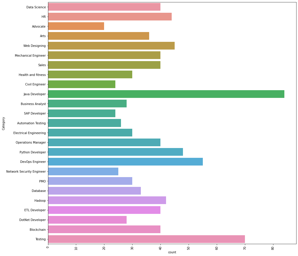
The output is generated.
Now, let us look at an individual entry to have a look how the data looks like.
df["Resume"][2]
Output:
'Areas of Interest Deep Learning, Control System Design, Programming in-Python, Electric Machinery, Web Development, Analytics Technical Activities q Hindustan Aeronautics Limited, Bangalore - For 4 weeks under the guidance of Mr. Satish, Senior Engineer in the hangar of Mirage 2000 fighter aircraft Technical Skills Programming Matlab, Python and Java, LabView, Python WebFrameWork-Django, Flask, LTSPICE-intermediate Languages and and MIPOWER-intermediate, Github (GitBash), Jupyter Notebook, Xampp, MySQL-Basics, Python Software Packages Interpreters-Anaconda, Python2, Python3, Pycharm, Java IDE-Eclipse Operating Systems Windows, Ubuntu, Debian-Kali Linux Education Details rnJanuary 2019 B.Tech. Electrical and Electronics Engineering Manipal Institute of TechnologyrnJanuary 2015 DEEKSHA CENTERrnJanuary 2013 Little Flower Public SchoolrnAugust 2000 Manipal Academy of HigherrnDATA SCIENCE rnrnDATA SCIENCE AND ELECTRICAL ENTHUSIASTrnSkill Details rnData Analysis- Exprience - Less than 1 year monthsrnexcel- Exprience - Less than 1 year monthsrnMachine Learning- Exprience - Less than 1 year monthsrnmathematics- Exprience - Less than 1 year monthsrnPython- Exprience - Less than 1 year monthsrnMatlab- Exprience - Less than 1 year monthsrnElectrical Engineering- Exprience - Less than 1 year monthsrnSql- Exprience - Less than 1 year monthsCompany Details rncompany - THEMATHCOMPANYrndescription - I am currently working with a Casino based operator(name not to be disclosed) in Macau.I need to segment the customers who visit their property based on the value the patrons bring into the company.Basically prove that the segmentation can be done in much better way than the current system which they have with proper numbers to back it up.Henceforth they can implement target marketing strategy to attract their customers who add value to the business.'
As we can see, the text needs a lot of processing. The is not suitable for analyzing, yet.
Data Cleaning
Now, we clean the text.
import re
def cleanResume(resumeText):
    resumeText = re.sub('httpS+s*', ' ', resumeText)  # remove URLs
    resumeText = re.sub('RT|cc', ' ', resumeText)  # remove RT and cc
    resumeText = re.sub('#S+', '', resumeText)  # remove hashtags
    resumeText = re.sub('@S+', '  ', resumeText)  # remove mentions
    resumeText = re.sub('[%s]' % re.escape("""!"#$%&'()*+,-./:;<=>?@[]^_`{|}~"""), ' ', resumeText)  # remove punctuations
    resumeText = re.sub(r'[^x00-x7f]',r' ', resumeText)
    resumeText = re.sub('s+', ' ', resumeText)  # remove extra whitespace
    return resumeText
df['Cleaned_Resume'] = df.Resume.apply(lambda x: cleanResume(x))
df.head()
Now, let us look at the data.

Now, we can see that the text is clean.
len(df)
Output: 962
So, there are 962 entries.
Now, we get the entire “Cleaned_Resume” as a single text.
#getting the entire resume text
corpus=" "
for i in range(0,962):
    corpus= corpus+ df["Cleaned_Resume"][i]
Let us now have a look at it.
corpus[1000:2500]
Output:
'review process and run analytics and generate reports Core member of a team helped in developing automated review platform tool from scratch for assisting E discovery domain this tool implements predictive coding and topic modelling by automating reviews resulting in reduced labor costs and time spent during the lawyers review Understand the end to end flow of the solution doing research and development for classification models predictive analysis and mining of the information present in text data Worked on analyzing the outputs and precision monitoring for the entire tool TAR assists in predictive coding topic modelling from the evidence by following EY standards Developed the classifier models in order to identify red flags and fraud related issues Tools Technologies Python scikit learn tfidf word2vec doc2vec cosine similarity Na ve Bayes LDA NMF for topic modelling Vader and text blob for sentiment analysis Matplot lib Tableau dashboard for reporting MULTIPLE DATA SCIENCE AND ANALYTIC PROJECTS USA CLIENTS TEXT ANALYTICS MOTOR VEHICLE CUSTOMER REVIEW DATA Received customer feedback survey data for past one year Performed sentiment Positive Negative Neutral and time series analysis on customer comments across all 4 categories Created heat map of terms by survey category based on frequency of words Extracted Positive and Negative words across all the Survey categories and plotted Word cloud Created customized tableau dashboards for effective reporting and visualizations CHAT'
As we see, the text has now been cleaned and joined together.
Tokenization
Now, we will Tokenize the words.
Tokenization is the process of breaking raw text into small units. Here, we convert the entire text into single words. Tokenization is important because it splits the data into small usable and easy-to-process units. These smaller units of text are called tokens. These tokens can help in understanding the context of the text and also in building the NLP models.
There are mainly 3 types of Tokenization: word, character, and subword (n-gram characters) tokenization. We use word tokenization for our analyzing purposes.
#Creating the tokenizer
tokenizer = nltk.tokenize.RegexpTokenizer('w+')
#Tokenizing the text
tokens = tokenizer.tokenize(corpus)
len(tokens)
Output: 411913
#now we shall make everything lowercase for uniformity
#to hold the new lower case words
words = []
# Looping through the tokens and make them lower case
for word in tokens:
    words.append(word.lower())
Everything is made into the lower case for uniformity. If this was not done, “Python” and “python” would be perceived as different which we don’t want.
StopWords
#Stop words are generally the most common words in a language.
#English stop words from nltk.
stopwords = nltk.corpus.stopwords.words('english')
words_new = []
#Now we need to remove the stop words from the words variable
#Appending to words_new all words that are in words but not in sw
for word in words:
    if word not in stopwords:
        words_new.append(word)
Here, we remove the stopwords from the text. For analyzing text and NLP, stopwords are removed from the text, as they do not add much value and meaning to the text. Stopwords, if added would bring in a lot of unnecessary noise and be of no use to the analytics process. Also, the removal of stopwords reduces the amount of data we have to process, thus reducing the number of tokens and makes everything faster.
Examples of Stopwords in English: ‘nor’, ‘me’, ‘were’, ‘her’, ‘more’, ‘himself’, ‘this’.
len(words_new)
Output: 318305
Lemmatization
Now, we proceed with Lemmatization. Lemmatization involves the process to group together the different forms of a word. This is done so as to analyze them as a single item. Lemmatization helps in consolidating various sentiments expressed in the text, which might imply or direct towards a similar response. Lemmatization usually returns a word to the base or dictionary form of a word. This form is known as the “lemma”.
To read more about Lemmatization, check out this article.
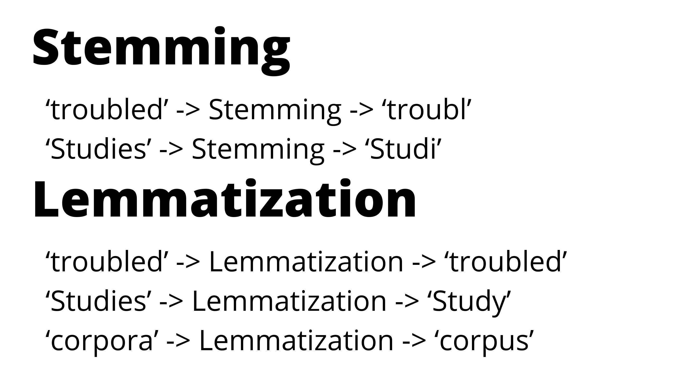
The code:
from nltk.stem import WordNetLemmatizer
wn = WordNetLemmatizer()
lem_words=[]
for word in words_new:
    word=wn.lemmatize(word)
    lem_words.append(word)
same=0
diff=0
for i in range(0,1832):
    if(lem_words[i]==words_new[i]):
        same=same+1
    elif(lem_words[i]!=words_new[i]):
        diff=diff+1
print('Number of words Lemmatized=', diff)
print('Number of words not Lemmatized=', same)
Output:
Number of words Lemmatized= 294
Number of words not Lemmatized= 1538
Now, with the Lemmatization done, we proceed to get the Frequency Distribution.
Frequency Distribution
#The frequency distribution of the words
freq_dist = nltk.FreqDist(lem_words)
#Frequency Distribution Plot
plt.subplots(figsize=(20,12))
freq_dist.plot(30)
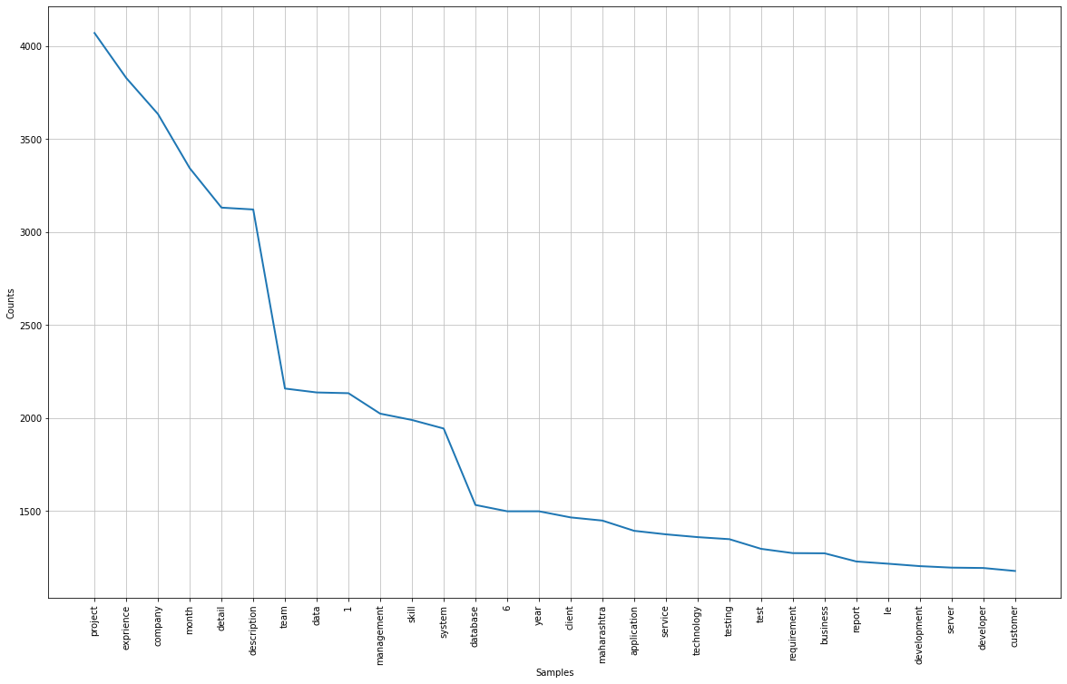
The visual might not be very clear here. I will leave the link to the code and dataset so that they can be viewed properly.
mostcommon = freq_dist.most_common(50)
mostcommon
Output:
[('project', 4071),
 ('exprience', 3829),
 ('company', 3635),
 ('month', 3344),
 ('detail', 3132),
 ('description', 3122),
 ('team', 2159),
 ('data', 2138),
 ('1', 2134),
 ('management', 2024),
 ('skill', 1990),
 ('system', 1944),
 ('database', 1533),
 ('6', 1499),
 ('year', 1499),
 ('client', 1466),
 ('maharashtra', 1449),
 ('application', 1394),
 ('service', 1375),
 ('technology', 1360),
 ('testing', 1349),
 ('test', 1297),
 ('requirement', 1274),
 ('business', 1273),
 ('report', 1229),
 ('le', 1217),
 ('development', 1204),
 ('server', 1196),
 ('developer', 1194),
 ('customer', 1178),
 ('ltd', 1177),
 ('process', 1163),
 ('responsibility', 1137),
 ('using', 1124),
 ('sql', 1120),
 ('january', 1090),
 ('java', 1076),
 ('engineering', 1055),
 ('work', 1038),
 ('pune', 1026),
 ('role', 969),
 ('c', 951),
 ('user', 916),
 ('operation', 895),
 ('software', 886),
 ('pvt', 879),
 ('sale', 845),
 ('activity', 832),
 ('environment', 800),
 ('design', 786)]
We can have a look at the frequency distribution, words like project, company, management, team, etc are very common. Having a look at the entire frequency table will show which types of words are more used.
Recruiters can apply these analytics to understand the general profile of the applicants. Often screening and applicant selection are done on metrics gathered from Resume text.
WordCloud
Now, we generate a word cloud.
#converting into string
res=' '.join([i for i in lem_words if not i.isdigit()])
plt.subplots(figsize=(16,10))
wordcloud = WordCloud(
                          background_color='black',
                          max_words=100,
                          width=1400,
                          height=1200
                         ).generate(res)
plt.imshow(wordcloud)
plt.title('Resume Text WordCloud (100 Words)')
plt.axis('off')
plt.show()
Output:
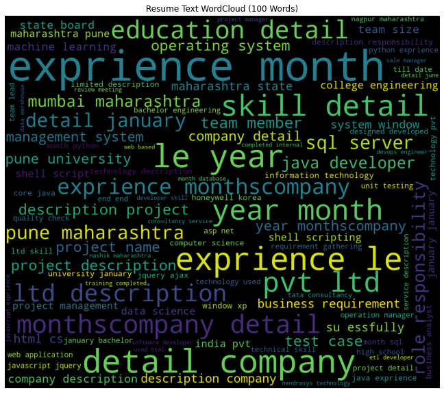
Now, we make the word cloud with the top 200 words.
plt.subplots(figsize=(20,15))
wordcloud = WordCloud(
                          background_color='black',
                          max_words=200,
                          width=1400,
                          height=1200
                         ).generate(res)
plt.imshow(wordcloud)
plt.title('Resume Text WordCloud (200 Words)')
plt.axis('off')
plt.show()
Output:
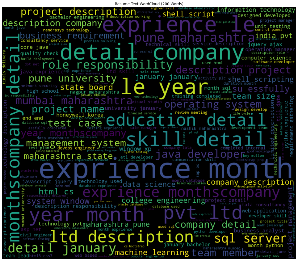
Word Clouds are an interesting text analytics tool. As the size of the words is determined by their frequency, by looking at the figure we can understand we understand which words are more important/ appear more times in the text. These are some of the simple, yet meaningful text analytics methods.
Now let us explore some words in the Data Science resumes.
data_science= df[df["Category"]=="Data Science"]
data_science.head()

len(data_science)
Output: 40
#getting the entire resume text
data_science_corpus=" "
for i in range(0,40):
    data_science_corpus= data_science_corpus+ data_science["Cleaned_Resume"][i]
data_science_corpus=data_science_corpus.lower()
Now, we split it into words to get word frequencies.
words_data_science=data_science_corpus.split()
Now, we try the frequencies of important terms in Data Science.
print('Frequency of "python"  is :', words_data_science.count("python"))
Frequency of "python"  is : 176
print('Frequency of "sap"  is :', words_data_science.count("sap"))
Frequency of "sap"  is : 68
print('Frequency of "analysis"  is :', words_data_science.count("analysis"))
Frequency of "analysis"  is : 84
print('Frequency of "sql"  is :', words_data_science.count("sql"))
Frequency of "sql"  is : 72
print('Frequency of "neural"  is :', words_data_science.count("neural"))
Frequency of "neural"  is : 48
print('Frequency of "network"  is :', words_data_science.count("network"))
Frequency of "network"  is : 12
print('Frequency of "networks"  is :', words_data_science.count("networks"))
Frequency of "networks"  is : 20
print('Frequency of "pandas"  is :', words_data_science.count("pandas"))
Frequency of "pandas"  is : 24
print('Frequency of "r"  is :', words_data_science.count("r"))
Frequency of "r"  is : 36
print('Frequency of "excel"  is :', words_data_science.count("excel"))
Frequency of "excel"  is : 12
print('Frequency of "anaconda"  is :', words_data_science.count("anaconda"))
Frequency of "anaconda"  is : 4
print('Frequency of "jupyter"  is :', words_data_science.count("jupyter"))
Frequency of "jupyter"  is : 4
print('Frequency of "education"  is :', words_data_science.count("education"))
Frequency of "education"  is : 48
print('Frequency of "experience"  is :', words_data_science.count("experience"))
Frequency of "experience"  is : 52
Thus, with text analytics, we were able to understand many aspects of the text.
We can see that Python appeared many times, which is a must-know language for Data Science.
Do check the code.
Final Words:
Text Analytics is an interesting area and needs a lot more work and research. With good Text Analytics, we are able to process a lot of text data and understand many things. In the above example, with text analytics, we are able to clean the text and gather valuable information regarding the resume texts.
About me:
Prateek Majumder
Data Science and Analytics | Digital Marketing Specialist | SEO | Content Creation
Connect with me on Linkedin.
My other articles on Analytics Vidhya: Link.
Thank You.
The media shown in this article on Sign Language Recognition are not owned by Analytics Vidhya and are used at the Author’s discretion.


