This article was published as a part of the Data Science Blogathon
Introduction
The main goal of this post is to compare the performance of the Pycaret and Cat boost library by solving a binary classification problem. Soccer, also known as football, is one of the most famous games in the world. If groups of people can pause time and make people watch them in wonder and love, it is this excellent game. Also, anyone can play this game – that needs four poles, a ground, and a ball. When Nelson Mandela was elected President of South Africa after the Apartheid era, he used football as a powerful unifier. The sport easily transcends all barriers to participation.
This lovely sport is the centre of an entire ecosystem. The amount of money involved in this game is incredible. It has an impact on millions of people who rely on it for a living and recreation. There are many Clubs, Merchandise, and a group of rivals based on the game outcome.
Today, our problem statement is a typical case study for making decisions and determining the odds in a given situation.
I guess most people are aware of these two libraries, and others can check out Pycaret, Catboost documentation for a better understanding.
Before solving our problem, here is a little brief about both of these libraries.
Pycaret has extensive applications in the field of Business Intelligence. It helps in creating end-to-end ML experiments, spend less time coding and focus on the business problems. PyCaret integrates with other tools like Tableau and PowerBI. It can be used in a variety of notebooks, including Jupyter, Google Colab, Azure Notebooks, and others.
Pycaret Features
- Faster preparation of data and model training.
- Easy tuning of Hyperparameters.
- Features and model results are easy to explore and interpretable.
- Faster model selection and experiment logging.
CatBoost is a decision tree gradient boosting technique. It was created by Yandex researchers and engineers and is used at Yandex and other organizations like CERN, Cloudflare, and Careem taxi for search, recommendation systems, personal assistants, self-driving cars, weather prediction, and many other activities. It’s free and open-source, and anyone can use it.
Catboost Features
- It provides good results with default parameters.
- It allows non-numeric factors without spending more time in preprocessing.
- For large datasets, you can use a multi-card configuration.
- Constructing models with novel gradient boosting schema reduce overfitting.
- CatBoost’s model applier allows you to quickly and efficiently apply your learned model to latency-critical operations.
What is Binary Classification?
Binary classification is the task of separating data into two groups in Machine Learning. Problems like determining the class of clients from two groups for marketing a product launch are real-world instances of binary classification. We wish to divide the samples into two categories in binary classification. When we classify samples into more than two categories, we have a challenge called multiclass classification.
To figure out which machine learning algorithm is ideal for binary classification, look at the implementation and assumptions of each algorithm that will help you figure out where you should use the algorithm. But, to make things easier for you, we solve the binary classification problem below using two libraries.
To predict the outcome of the game, we have features such as ‘season’, ‘date’, ‘league_id’, ‘league’, ‘Team 1’, ‘Team2’, ‘SPI1’, ‘SPI2’, ‘proj_score1’, ‘proj_score2’, ‘importance1’, ‘importance2’, ‘score1’, ‘score2’, ‘xg1’, ‘xg2’, ‘nsxg1’, ‘nsxg2’, ‘adj_score1’, ‘adj_score2’, ‘Outcome’.
train.isna().sum()
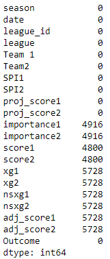
Ten features from the above mentioned have more than 30 per cent of missing values. We drop all those features, but one can substitute based on your choice.
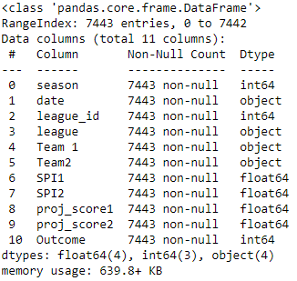
We have six numeric and three categorical, one date feature to predict our target Outcome.
Pycaret Approach
Importing Libraries
from pycaret.classification import *
import pandas as pd
train.shape
>(7443, 11)
test.shape
>(4008, 20)
train.head()

After dropping the columns with Na more than thirty per cent.
train.info()
Setting up the environment
exp = setup(data = train, target = 'Outcome', feature_selection=True,
            normalize = True, transformation = True, ignore_low_variance = True,
            remove_multicollinearity = True, multicollinearity_threshold = 0.95,)
In this approach, we use parameters such as feature_selection, normalize, transformation, ignore_low_variance, multicollinearity with a threshold of .95.
Here we use the compare models function we get the best performing model out of all the classification models.
compare_models()
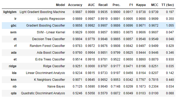
Above you can see the results, where the LGBM classifier performs well with an accuracy of 98 percent.
We create a Light gradient boost model to predict the outcome of test data since it has the highest accuracy.
# Creating the best model from above result
lgbm = create_model('lightgbm')
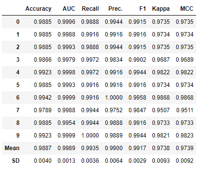
Below you can see the predicted results of test data outcome by using the predict_model function.
predict_model(lgbm, test)

Now, using the save_model() function helps to save the trained model for future use.
Catboost Approach
Make sure that you had installed the cat boost library and import the necessary libraries use.
Importing Libraries
import catboost
from catboost import CatBoostClassifier, cv, Pool
from sklearn.metrics import log_loss
from sklearn.model_selection import train_test_split
We exclude date, league features and create a list with remaining and a list of categorical features.
features = ['season','league_id', 'Team 1', 'Team2', 'SPI1', 'SPI2', 'proj_score1', 'proj_score2',]
cat_features = ['league_id', 'Team 1', 'Team2']
X = train[features]
y = train['Outcome']
Now, we use the train_test_split function from sklearn to split the data into training and validations sets.
X_train, X_valid, y_train, y_valid = train_test_split(X, y, train_size=0.8, random_state=SEED)
X_test = test[features]
We create a pool of data and define cat boost parameters for the model.
train_data = Pool(data=X_train, label=y_train, cat_features=cat_features)
valid_data = Pool(data=X_valid, label=y_valid, cat_features=cat_features)
The parameters used for model creation
CATBOOST_PARAMS = {'random_seed':SEED,'learning_rate':0.3,'iterations':175,
    'loss_function':'Logloss','max_depth':6,'early_stopping_rounds':10,'min_data_in_leaf':10}
Now, fit the model with train and validation data.
model = CatBoostClassifier(**CATBOOST_PARAMS)
model.fit(train_data, eval_set=(valid_data), use_best_model=True,
         logging_level= 'Silent',  #'Verbose',  # uncomment this for text output
         plot=True
        )
After fitting the model with training data, we use the validation data and observe the log_loss score for predicted values and probabilities.
log_loss(y_valid, model.predict(X_valid))
> 0.2551603335936137
log_loss(y_valid, model.predict_proba(X_valid))
> 0.03284821982060608
We use the randomized search, define parameters for the function with an iteration of 175, and users can play around with the parameters.
grid = {'learning_rate': [0.3, 0.5, 0.4, 0.1],
        'max_depth': [4,  6,  8,  10],
        'l2_leaf_reg': [1,  3,  5,  7, 9],
       }
model = CatBoostClassifier(iterations=175)
randomized_search_result = model.randomized_search(grid,
            X=all_train_data,
            cv=5,
            partition_random_seed=SEED,
            search_by_train_test_split=True,
            refit=True,
            shuffle=True,
            stratified=None,
            train_size=0.8,
            verbose=0,
            plot=False)
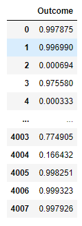
At last, we use the predict_proba function to get the probabilities of our test data.
preds = model.predict_proba(X_test)
Trick
To decrease log_loss, clip the values by using the below range. This will helps to boost the score on the leaderboard, but it doesn’t help us in all the scenarios.
We use log_loss as our evaluation metric for this binary classification problem. For submission, using the Pycaret result, we achieved a score of 0.2, and the catboost resulted in a score of 0.04.
Competition Winner Approach (Bonus)
The preprocessing techniques used:
- dropping the unusable features that have only missing values in test data.
- The month, weekday of the match, and sign of projective score difference is new extracted features
- drop outliers based on the last engineered features.
In EDA, the difference in projective scores was very informative. For the observations with a positive difference of projective scores, the outcome was 1 in 98.8% cases(only 6 has the Outcome of 0). At the same time, observations with a negative difference of projective scores have an Outcome of 0 in 99.8%(only 3 with one as Outcome). The goal difference of the opponents for the day is a newly created feature. After adding the new feature, the Decision Tree model.
Conclusion
Based on the evaluation metric, we can conclude Catboost performed better than Pycaret. But both libraries have their pros and cons. The tuning of hyperparameters and preprocessing might help to boost the performance of pycaret. The results depend on the preprocessing and feature engineering techniques used for the data. From the above winner approach, we can understand the importance of the difference between features. Finally, the more you explore, analyze data, extract new features and understand the business problem, you can create a robust model.
I hope you have found this post insightful, and have a great day. Thank you.


