Introduction
PCA, or Principal Component Analysis, is a term that is well-known to everyone. Notably employed for Curse of Dimensionality issues. In addition to this fundamental issue, there are other significant issues that we tackle in the PCA article. So, let’s start with fundamental knowledge. In this article, I’ve also added my handwritten manual technique for PCA in machine learning, layman comprehension, some key theory, and a Python approach.
This article was published as a part of the Data Science Blogathon.
Table of contents
- Introduction
- Principal Component Analysis (PCA) in Machine Learning?
- Why Do We Need PCA in Machine Learning?
- Dimensionality Reduction Work in Real-Time Application
- Basic Terminologies of PCA
- How does PCA work?
- Advantage for Principal Component Analysis
- Disadvantage for Principal Component Analysis
- Application for Principal Component Analysis
- Python Code for Principal Component Analysis
- Conclusion
- Frequently Asked Questions
Principal Component Analysis (PCA) in Machine Learning?
- PCA can be abbreviated as Principal Component Analysis
- PCA comes under the Unsupervised Machine Learning category
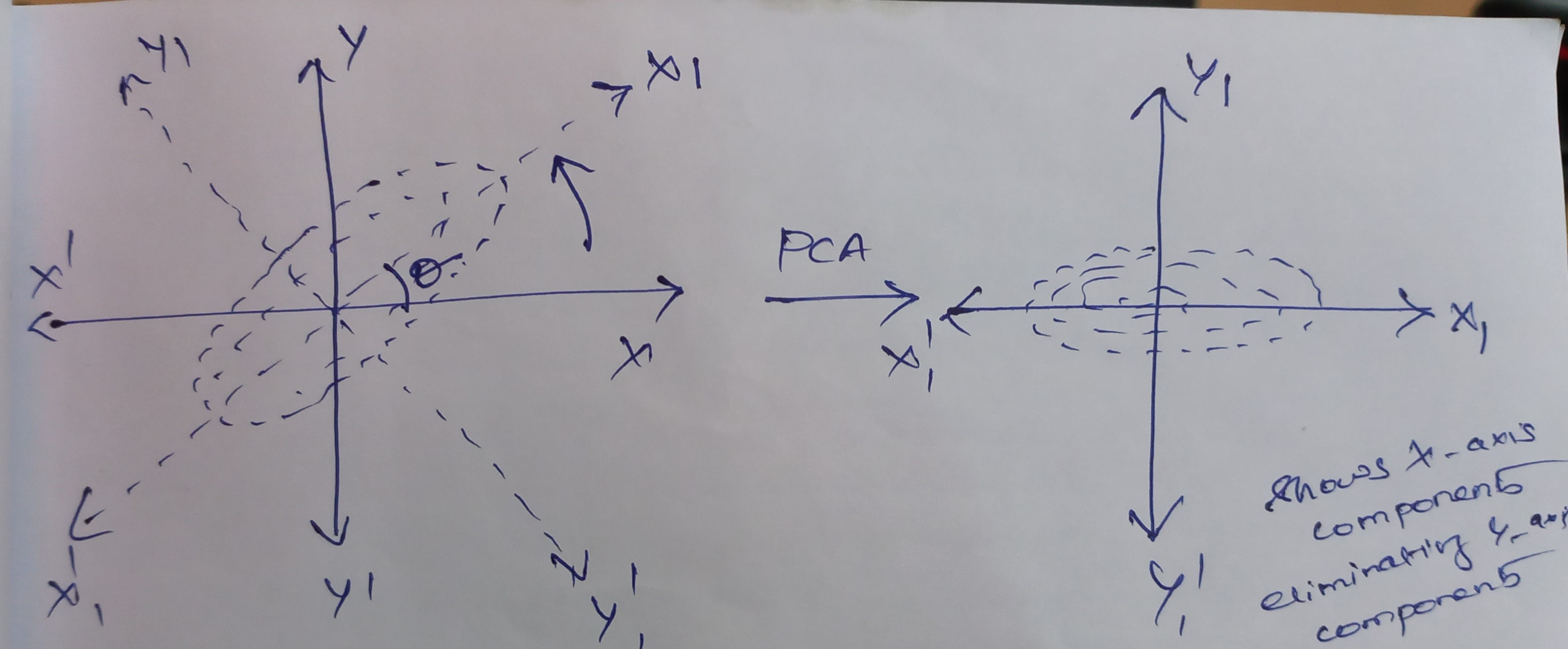
- Reducing the number of variables in a data collection while retaining as much information as feasible is the main goal of PCA. PCA can be mainly used for Dimensionality Reduction and also for important feature selection.
- Correlated features to Independent features
Technically, PCA provides a complete explanation of the composition of variance and covariance using multiple linear combinations of the core variables. Row scattering may be analyzed using PCA, which also identifies the distribution-related properties.
Why Do We Need PCA in Machine Learning?
When a computer is trained on a big, well-organized dataset, machine learning often excels. One of the techniques used to handle the curse of dimensionality in machine learning is principal component analysis (PCA). Typically, having a sufficient amount of data enables us to create a more accurate prediction model since we have more data to use to train the computer. But working with a huge data collection has its own drawbacks. The curse of dimensionality is the ultimate trap.
The title of an unreleased Harry Potter novel does not refer to what happens when your data has too many characteristics and perhaps not enough data points; rather, it refers to the curse of dimensionality. One can use dimensionality reduction to escape the dimensionality curse. Having 50 variables may be cut down to 40, 20, or even 10. The strongest effects of dimensionality reduction are found here.
Overfitting issues will arise while working with high-dimensional data, and dimensionality reduction will be used to address them. Increasing interpretability and minimizing information loss. aids in locating important characteristics. Aids in the discovery of a linear combination of varied sequences.
When to use PCA?
- Whenever we need to know our features are independent of each other
- Whenever we need fewer features from higher features
Dimensionality Reduction Work in Real-Time Application
Assume there are 50 questions in all in the survey. The following three are among them: Please give the following a rating between 1 and 5:
- I feel comfortable around people
- I easily make friends
- I like going out
These queries could appear different now. There is a catch, though. They aren’t, generally speaking. They all gauge how extroverted you are. Therefore, combining them makes it logical, right? That’s where linear algebra and dimensionality reduction methods come in! We want to lessen the complexity of the problem by minimizing the number of variables since we have much too many variables that aren’t all that different. That is the main idea behind dimensionality reduction. And it just so happens that PCA is one of the most straightforward and popular techniques in this field. As a general guideline, maintain at least 70–80 percent of the explained variation.
Intuition behind PCA
Let’s assume we are playing a mind game here like,
| Person | Height |
| A | 145 |
| B | 160 |
| C | 185 |
from the above table, we need to find the tallest person.

I can by seeing person A is the tallest. Now change the scenario
| Person | Height |
| D | 172 |
| E | 173 |
| F | 171 |
Can you guess who’s who? It’s tough when they are very similar in height.

Because of how much their heights vary, we previously had no issue telling a 185cm person from a 160cm and a 145cm person. Similar to this, our data contains more information when its variance is bigger. This explains why the terms PCA and maximum variance are frequently used together.
Basic Terminologies of PCA
Before getting into PCA, we need to understand some basic terminologies,
- Variance – for calculating the variation of data distributed across dimensionality of graph
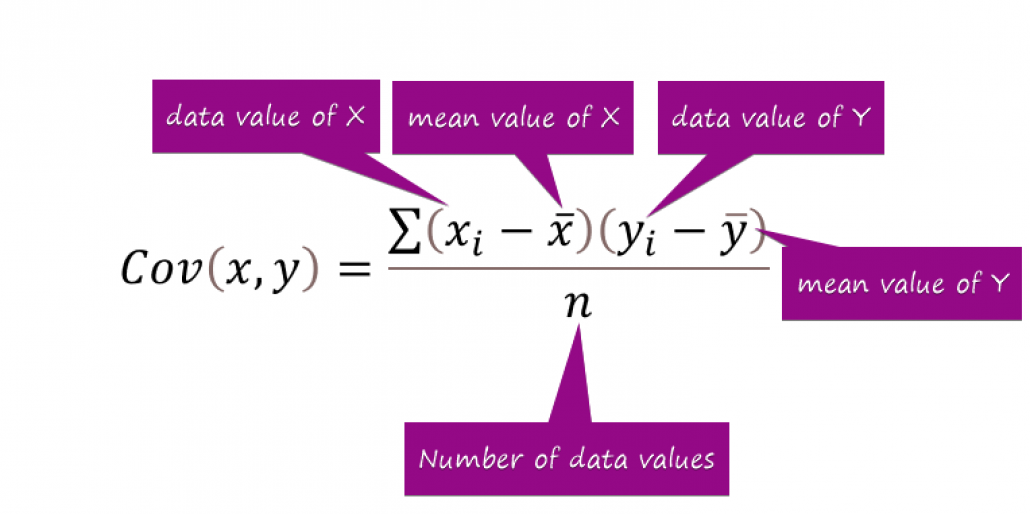
- Covariance – calculating dependencies and relationship between features
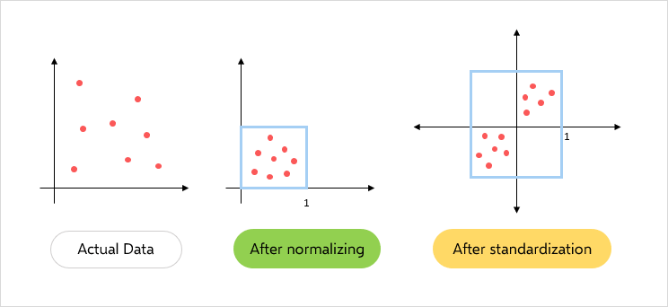
- Standardizing data – Scaling our dataset within a specific range for unbiased output
- Covariance matrix – Used for calculating interdependencies between the features or variables and also helps in reduce it to improve the performance
- EigenValues and EigenVectors – Eigenvectors’ purpose is to find out the largest variance that exists in the dataset to calculate Principal Component. Eigenvalue means the magnitude of the Eigenvector. Eigenvalue indicates variance in a particular direction and whereas eigenvector is expanding or contracting X-Y (2D) graph without altering the direction.
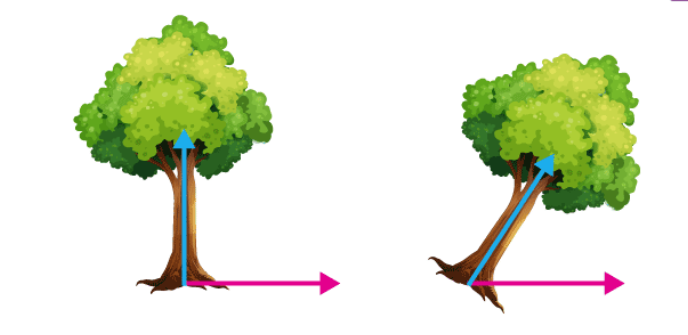
In this shear mapping, the blue arrow changes direction whereas the pink arrow does not. The pink arrow in this instance is an eigenvector because of its constant orientation. The length of this arrow is also unaltered, and its eigenvalue is 1. Technically, PC is a straight line that captures the maximum variance (information) of the data. PC shows direction and magnitude. PC are perpendicular to each other.
- Dimensionality Reduction – Transpose of original data and multiply it by transposing of the derived feature vector. Reducing the features without losing information.

How does PCA work?
The steps involved for PCA are as follows-
- Original Data
- Normalize the original data (mean =0, variance =1)
- Calculating covariance matrix
- Calculating Eigen values, Eigen vectors, and normalized Eigenvectors
- Calculating Principal Component (PC)
- Plot the graph for orthogonality between PCs
I have solved through manually, and the importance of hand-written notes is getting the crux behind the coding concepts,
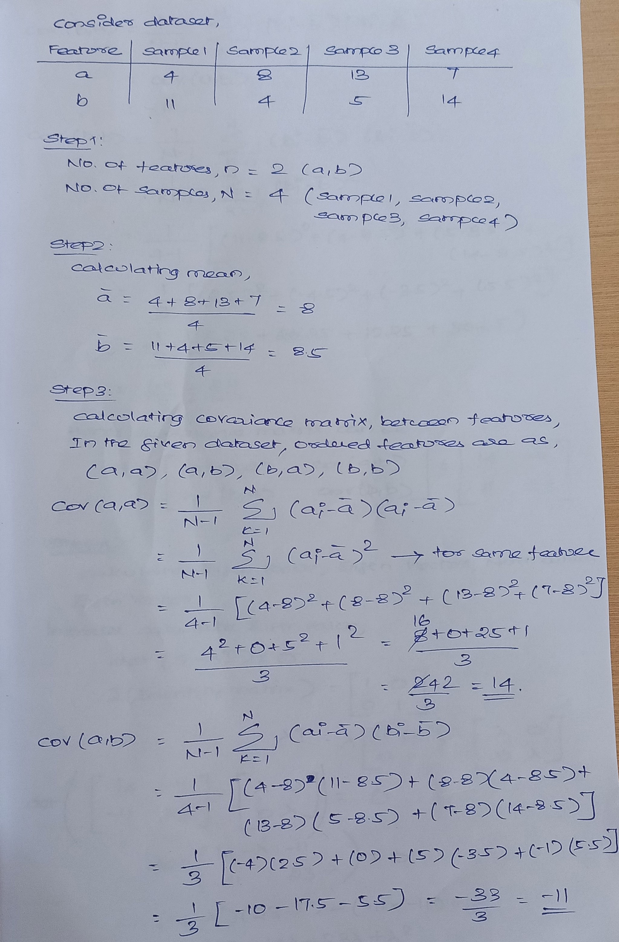
We are calculating means and then calculating the covariance matrix between features.
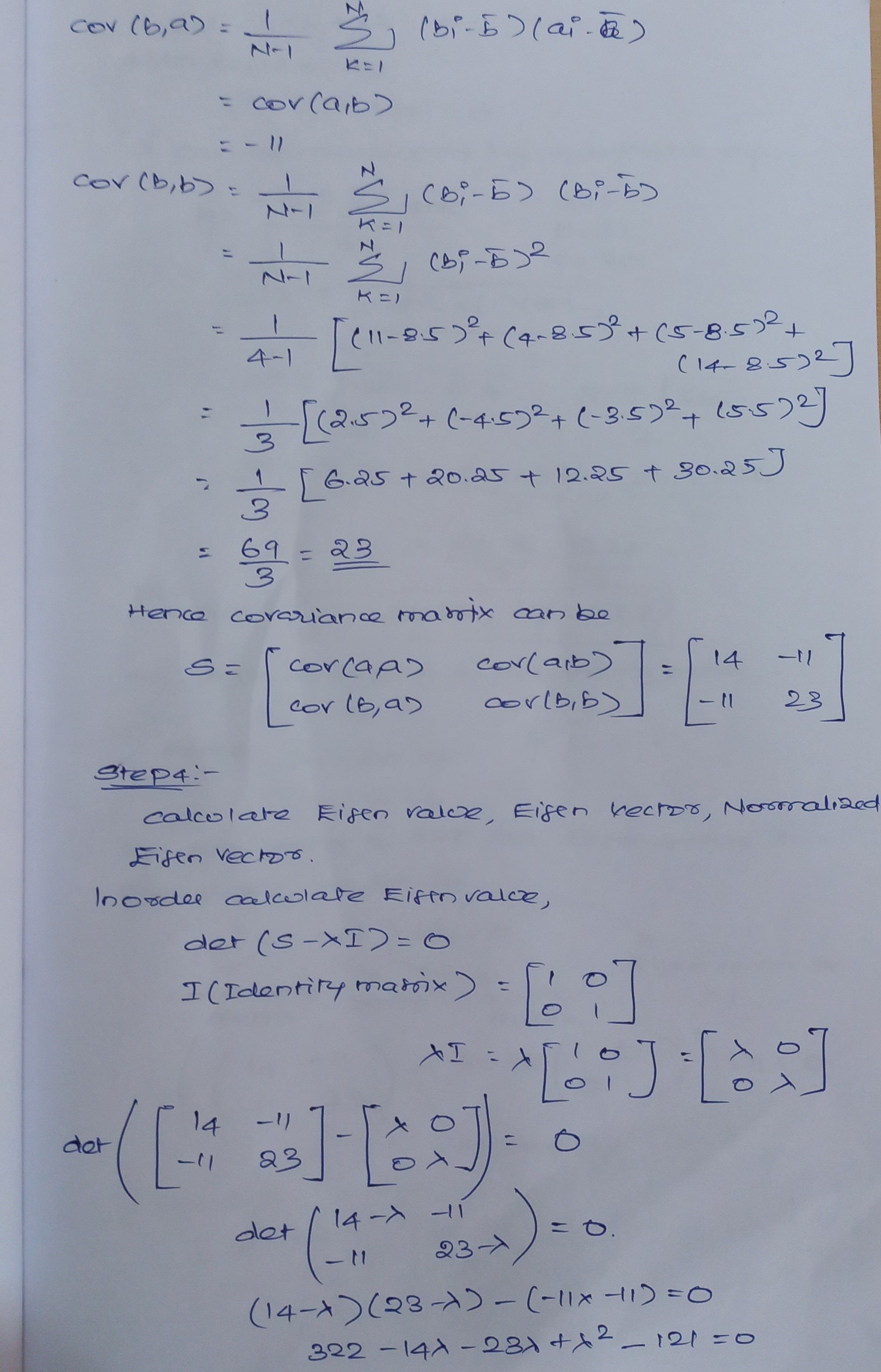
After finding covariance matrix, we are going to calculate the eigenvalue, eigenvector, and normalized eigenvector
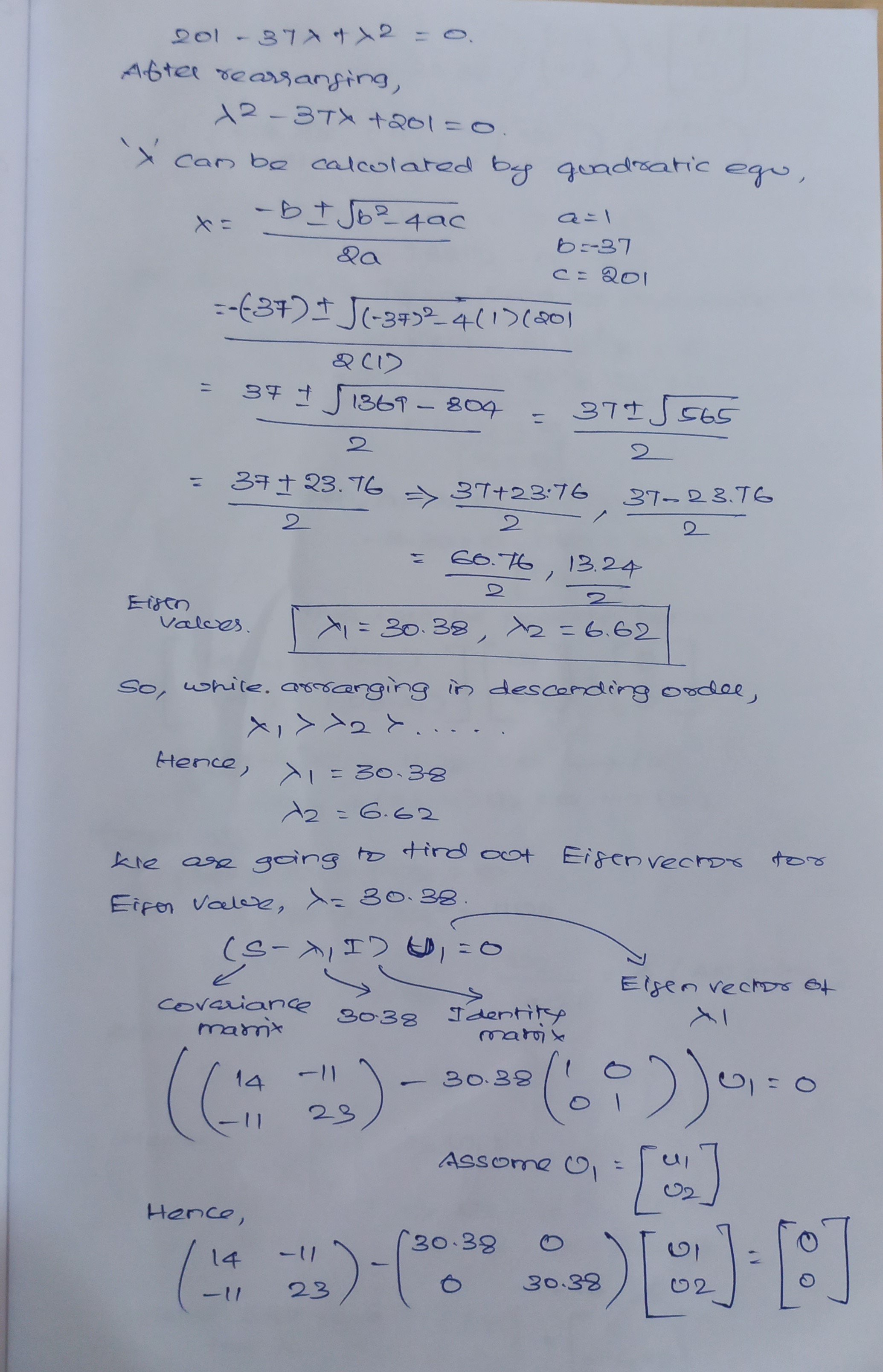
Steps involved in eigenvalues and vectors, in the manual approach
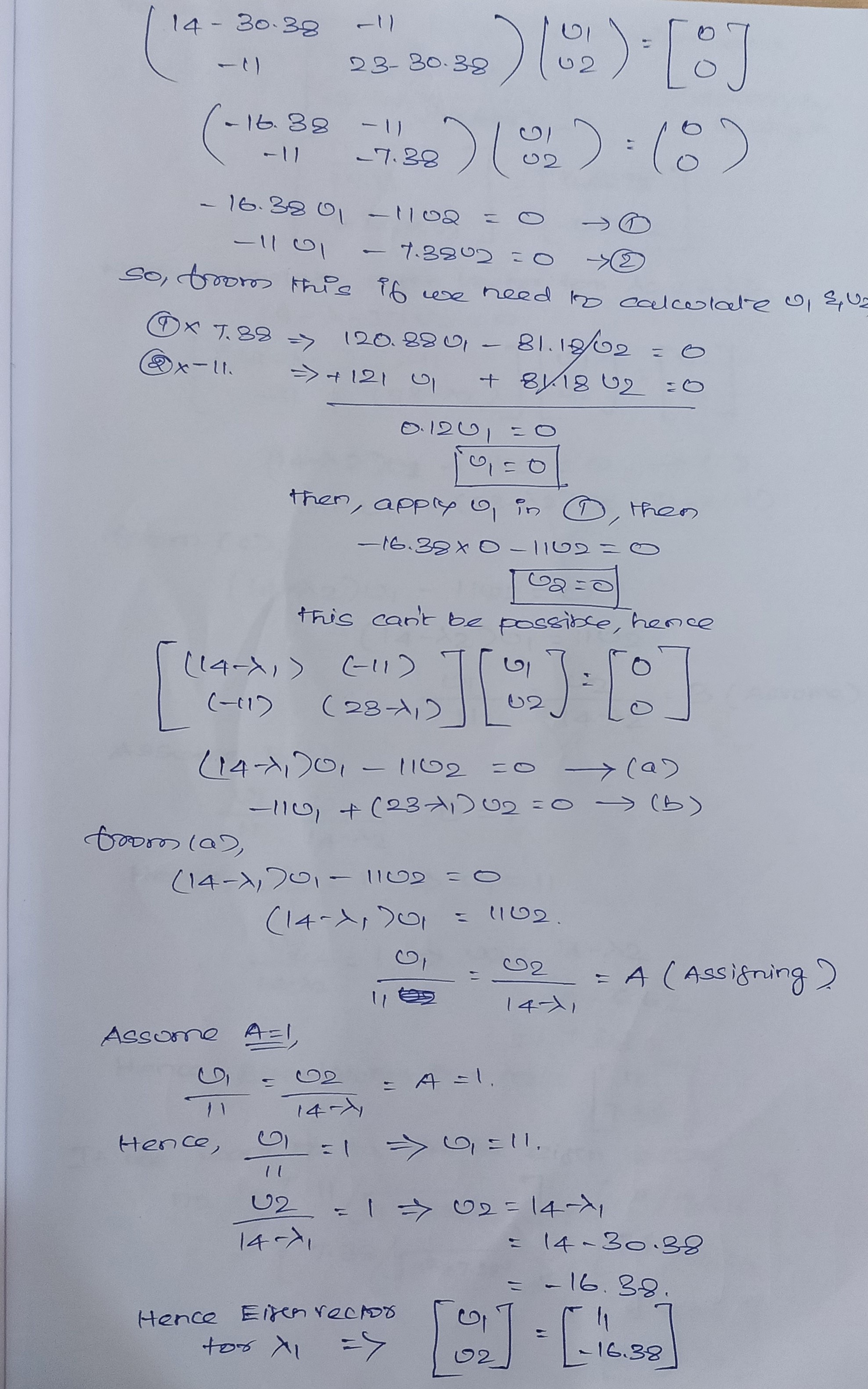
From this, we are going to calculate PCs
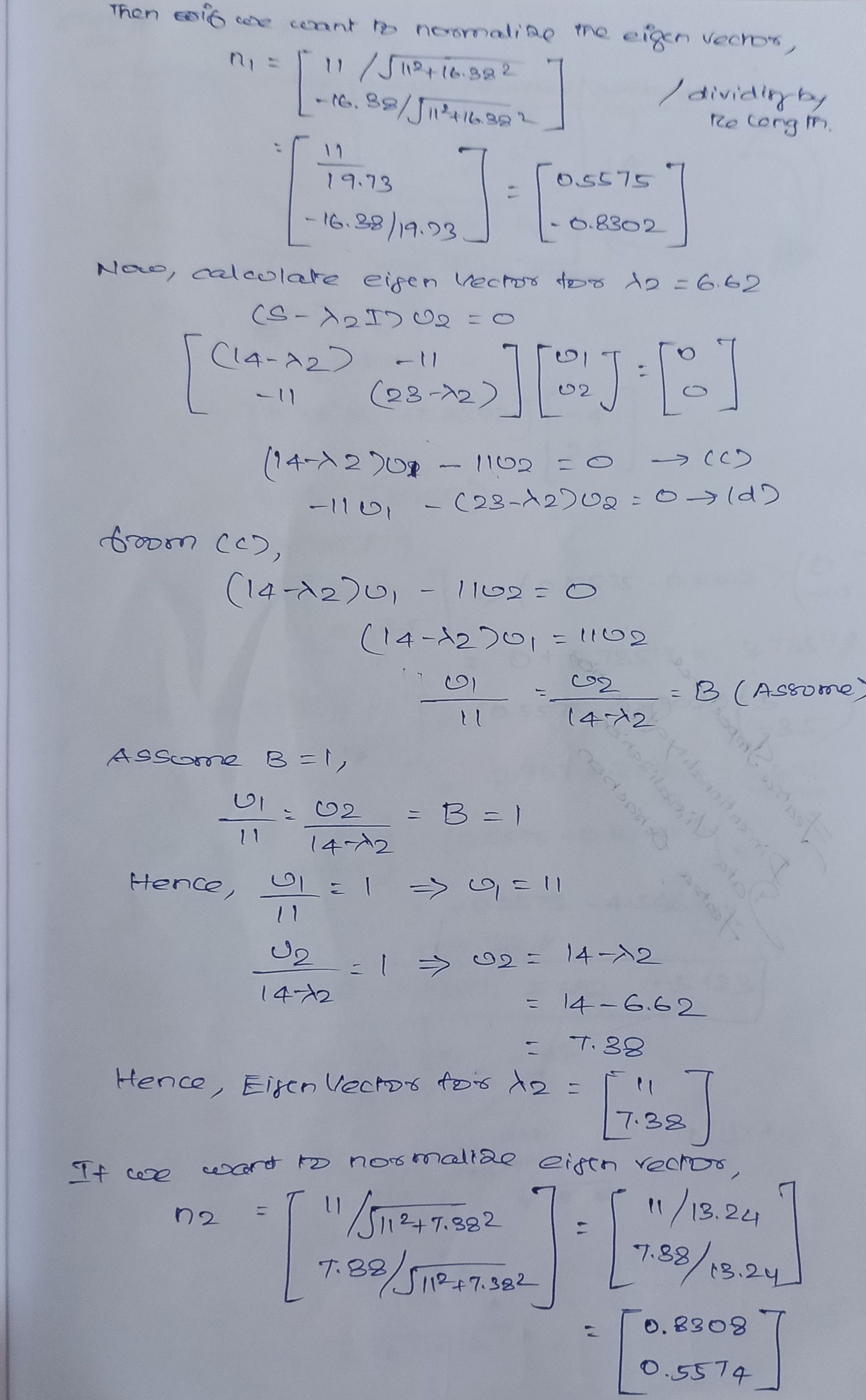
We are going to calculate the normalized eigenvector
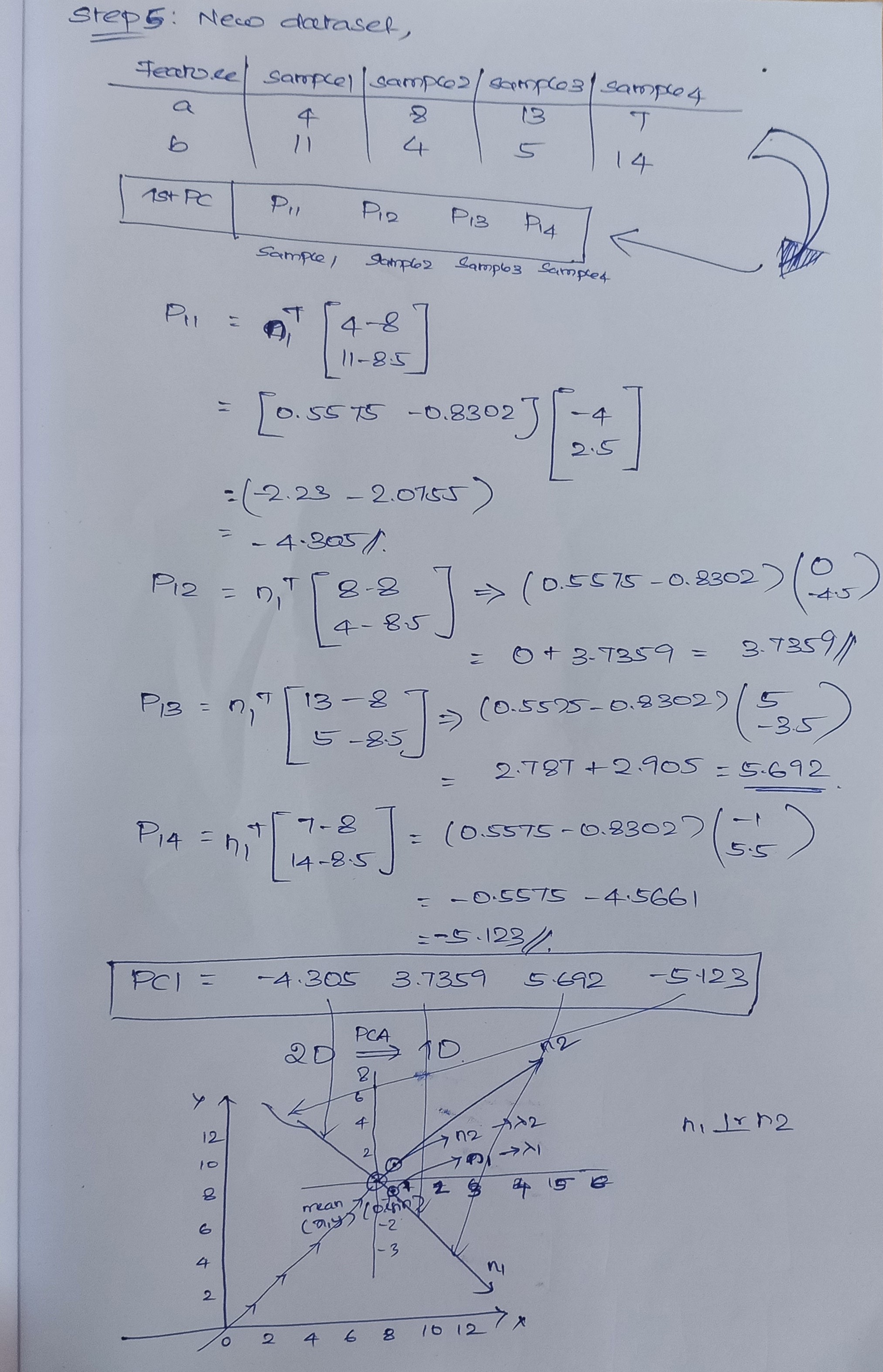
Hence PCA is calculated and visually we can see how PC are orthogonal to each other.
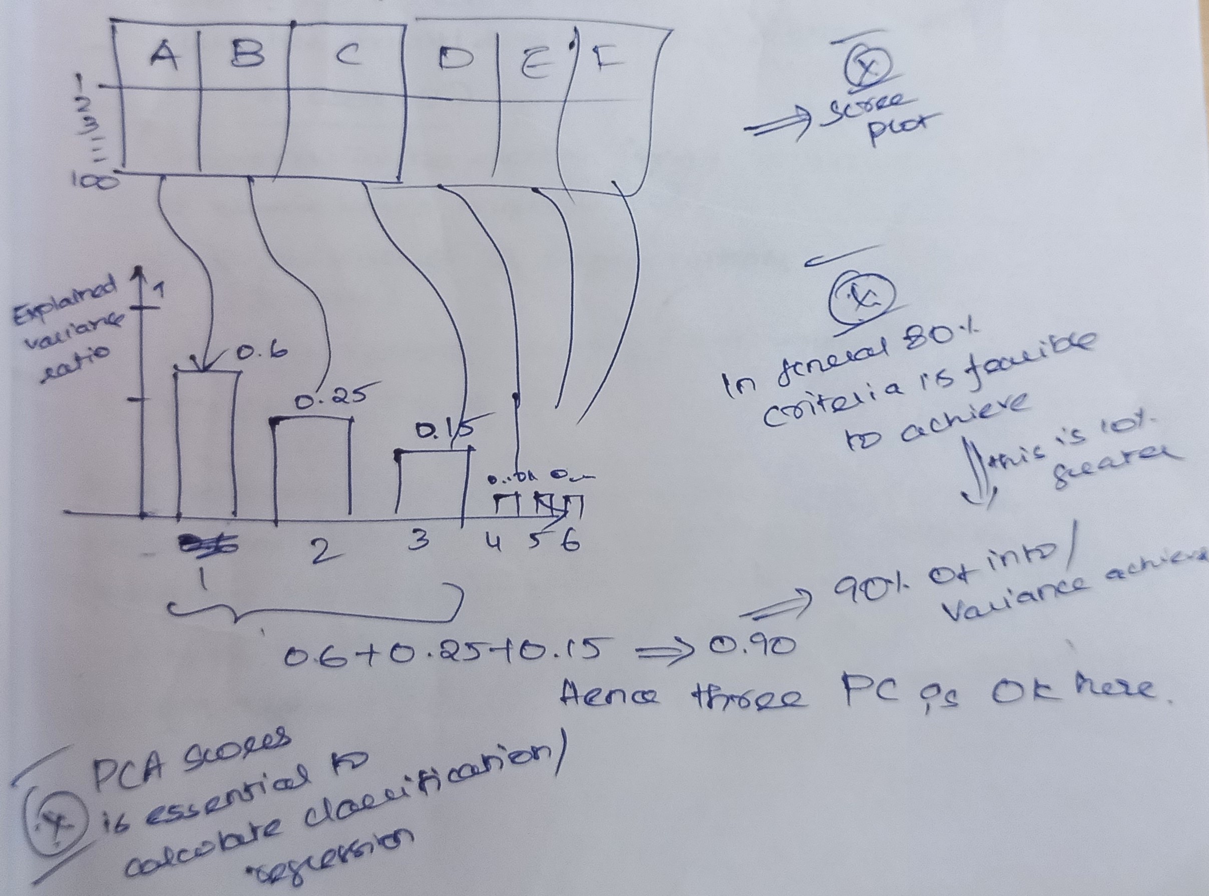
How Many PCAs are Needed for Any Data?
PCA has maximum variance (information), which will be good to select.
Eigenvalues are used to find out which PCA has a maximum variance.
Advantage for Principal Component Analysis
- Used for Dimensionality Reduction
- PCA will assist you in eliminating all related features, sometimes referred to as multi-collinearity.
- The time required to train your model is now substantially shorter because to PCA’s reduction in the number of features.
- PCA aids in overcoming overfitting by eliminating the extraneous features from your dataset.
Disadvantage for Principal Component Analysis
- Useful for quantitative data but not effective with qualitative data.
- Interpretation of PC is difficult from original data
Application for Principal Component Analysis
- Computer Vision
- Bio-informatics application
- For compressed images or resizing of the image
- Discovering patterns from high-dimensional data
- Reduction of dimensions
- Multidimensional Data – Visualization
Python Code for Principal Component Analysis
Before working with any dataset, let’s try it with some randomly generated data:
rng = np.random.RandomState(1)
X = np.dot(rng.rand(2, 2), rng.randn(2, 200)).T
plt.scatter(X[:, 0], X[:, 1])
plt.axis('equal');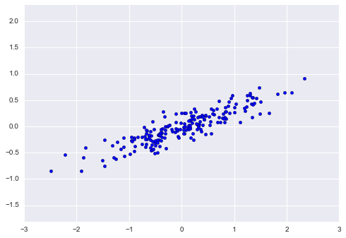
from sklearn.decomposition import PCA
pca = PCA(n_components=2)
pca.fit(X)
print(pca.components_)
print(pca.explained_variance_)

def draw_vector(v0, v1, ax=None):
    ax = ax or plt.gca()
    arrowprops=dict(arrowstyle='->',
                    linewidth=2,
                    shrinkA=0, shrinkB=0)
    ax.annotate('', v1, v0, arrowprops=arrowprops)

# plot data
plt.scatter(X[:, 0], X[:, 1], alpha=0.2)
for length, vector in zip(pca.explained_variance_, pca.components_):
    v = vector * 3 * np.sqrt(length)
    draw_vector(pca.mean_, pca.mean_ + v)
plt.axis('equal');

pca = PCA(n_components=1)
pca.fit(X)
X_pca = pca.transform(X)
print("original shape:   ", X.shape)
print("transformed shape:", X_pca.shape)

X_new = pca.inverse_transform(X_pca)
plt.scatter(X[:, 0], X[:, 1], alpha=0.2)
plt.scatter(X_new[:, 0], X_new[:, 1], alpha=0.8)
plt.axis('equal');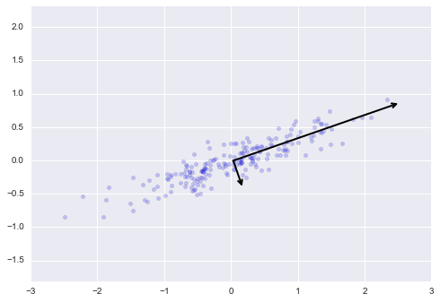
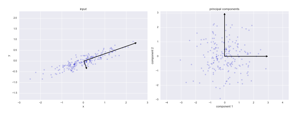
These vectors represent the principal axes of the data, and the length of the vector is an indication of how “important” that axis is in describing the distribution of the data—more precisely, it is a measure of the variance of the data when projected onto that axis. The projection of each data point onto the principal axes are the “principal components” of the data.
If we plot these principal components besides the original data, we see the plots shown here:
pca = PCA(n_components=1)
pca.fit(X)
X_pca = pca.transform(X)
print("original shape:   ", X.shape)
print("transformed shape:", X_pca.shape)
One dimension now exists for the converted data. We can run the inverse transform on this reduced data and display it next to the original data to visualize the impact of this dimensionality reduction:
X_new = pca.inverse_transform(X_pca)
plt.scatter(X[:, 0], X[:, 1], alpha=0.2)
plt.scatter(X_new[:, 0], X_new[:, 1], alpha=0.8)
plt.axis('equal');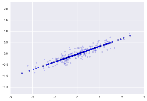
The actual data is represented by the bright dots, while the projected data is shown by the dark points. This explains what is meant by a PCA dimensionality reduction: the data along the primary axis(es) that are least relevant are deleted, leaving only the component(s) of the data that have the largest variance. The amount of “information” lost in this decrease of dimensionality is generally measured by the proportion of variance that is eliminated.
For better understanding, we are working with the default pre-loaded dataset called breast cancer.
from sklearn.datasets import load_breast_cancer
breast_cancer = load_breast_cancer()

print(breast_cancer.feature_names)
print(len(breast_cancer.feature_names))

import numpy as np
print(breast_cancer.target)
print(breast_cancer.target_names)
print(np.array(np.unique(breast_cancer.target, return_counts=True)))


import numpy as np
import matplotlib.pyplot as plt
_, axes = plt.subplots(6,5, figsize=(15, 15))
malignant = breast_cancer.data[breast_cancer.target==0]
benign = breast_cancer.data[breast_cancer.target==1]
ax = axes.ravel()                     # flatten the 2D array
for i in range(30):                   # for each of the 30 features
    bins = 40

    #---plot histogram for each feature---
    ax[i].hist(malignant[:,i], bins=bins, color='r', alpha=.5)
    ax[i].hist(benign[:,i], bins=bins, color='b', alpha=0.3)
    #---set the title---
    ax[i].set_title(breast_cancer.feature_names[i], fontsize=12)

    #---display the legend---
    ax[i].legend(['malignant','benign'], loc='best', fontsize=8)
plt.tight_layout()
plt.show()
import pandas as pd
df = pd.DataFrame(breast_cancer.data,
                  columns = breast_cancer.feature_names)
df['diagnosis'] = breast_cancer.target
df

#Training the Model using all the Features
from sklearn.linear_model import LogisticRegression
from sklearn.model_selection import train_test_split
X = df.iloc[:,:-1]
y = df.iloc[:,-1]
#---perform a split---
random_state = 12
X_train, X_test, y_train, y_test =
    train_test_split(X, y,
                     test_size = 0.3,
                     shuffle = True,
                     random_state=random_state)

#---train the model using Logistic Regression---
log_reg = LogisticRegression(max_iter = 5000)
log_reg.fit(X_train, y_train)
#---evaluate the model---
log_reg.score(X_test,y_test)

#Training the Model using Reduced Features
df_corr = df.corr()['diagnosis'].abs().sort_values(ascending=False)
df_corr
# get all the features that has at least 0.6 in correlation to the
# target
features = df_corr[df_corr > 0.6].index.to_list()[1:]
features                          # without the 'diagnosis' column

#Checking for MultiCollinearity
import pandas as pd
from sklearn.linear_model import LinearRegression
def calculate_vif(df, features):
    vif, tolerance = {}, {}
    # all the features that you want to examine
    for feature in features:
        # extract all the other features you will regress against
        X = [f for f in features if f != feature]
        X, y = df[X], df[feature]

        # extract r-squared from the fit
        r2 = LinearRegression().fit(X, y).score(X, y)
        # calculate tolerance
        tolerance[feature] = 1 - r2
        # calculate VIF
        vif[feature] = 1/(tolerance[feature])

    # return VIF DataFrame
    return pd.DataFrame({'VIF': vif, 'Tolerance': tolerance})
calculate_vif(df,features)
# try to reduce those feature that has high VIF until each feature
# has VIF less than 5
features = [
    'worst concave points',
    'mean radius',
    'mean concavity',
]
calculate_vif(df,features)
#Training the Model
from sklearn.linear_model import LogisticRegression
from sklearn.model_selection import train_test_split
X = df.loc[:,features]            # get the reduced features in the
                                  # dataframe
y = df.loc[:,'diagnosis']

# perform a split
X_train, X_test, y_train, y_test =
    train_test_split(X, y,
                     test_size = 0.3,
                     shuffle = True,
                     random_state=random_state)
log_reg = LogisticRegression()
log_reg.fit(X_train, y_train)
log_reg.score(X_test,y_test)

#Training the Model using Reduced Features (PCA)
#Performing Standard Scaling
from sklearn.preprocessing import StandardScaler
# get the features and label from the original dataframe
X = df.iloc[:,:-1]
y = df.iloc[:,-1]

# performing standardization
sc = StandardScaler()
X_scaled = sc.fit_transform(X)

#Applying Principal Component Analysis (PCA)

from sklearn.decomposition import PCA
components = None
pca = PCA(n_components = components)
# perform PCA on the scaled data
pca.fit(X_scaled)

# print the explained variances
print("Variances (Percentage):")
print(pca.explained_variance_ratio_ * 100)
print()
print("Cumulative Variances (Percentage):")
print(pca.explained_variance_ratio_.cumsum() * 100)
print()

# plot a scree plot
components = len(pca.explained_variance_ratio_)
    if components is None else components
plt.plot(range(1,components+1),
         np.cumsum(pca.explained_variance_ratio_ * 100))
plt.xlabel("Number of components")
plt.ylabel("Explained variance (%)")
from sklearn.decomposition import PCA
pca = PCA(n_components = 0.85)
pca.fit(X_scaled)
print("Cumulative Variances (Percentage):")
print(np.cumsum(pca.explained_variance_ratio_ * 100))
components = len(pca.explained_variance_ratio_)
print(f'Number of components: {components}')

# Make the scree plot
plt.plot(range(1, components + 1), np.cumsum(pca.explained_variance_ratio_ * 100))
plt.xlabel("Number of components")
plt.ylabel("Explained variance (%)")
pca_components = abs(pca.components_)
print(pca_components)

print('Top 4 most important features in each component')
print('===============================================')
for row in range(pca_components.shape[0]):
    # get the indices of the top 4 values in each row
    temp = np.argpartition(-(pca_components[row]), 4)
    # sort the indices in descending order
    indices = temp[np.argsort((-pca_components[row])[temp])][:4]
    # print the top 4 feature names
    print(f'Component {row}: {df.columns[indices].to_list()}')

#Transforming all the 30 Columns to the 6 Principal Components
X_pca = pca.transform(X_scaled)
print(X_pca.shape)
print(X_pca)

#Creating a Machine Learning Pipeline

from sklearn.pipeline import Pipeline
from sklearn.preprocessing import StandardScaler
from sklearn.decomposition import PCA
from sklearn.linear_model import LogisticRegression
_sc = StandardScaler()
_pca = PCA(n_components = components)
_model = LogisticRegression()
log_regress_model = Pipeline([
    ('std_scaler', _sc),
    ('pca', _pca),
    ('regressor', _model)
])

# perform a split
X_train, X_test, y_train, y_test =
    train_test_split(X, y,
                     test_size=0.3,
                     shuffle=True,
                     random_state=random_state)

# train the model using the PCA components
log_regress_model.fit(X_train,y_train)
log_regress_model.score(X_test,y_test)
Conclusion
I anticipate that the learners now have some understanding of Principal Component Analysis, the most important method in unsupervised machine learning. Principal Component Analysis is used for more than simply dimension reduction; it may also be used to identify key characteristics and solve multicollinearity issues. Although the knowledge I’ve provided here is important and useful for the projects we’ll be using, there are still a lot of things we need to understand. In upcoming columns, I’ll be disclosing. Coding and theory by themselves won’t make any issue easier to comprehend. Because of this, I also included handwritten comments.
Frequently Asked Questions
A. PC1 and PC2 in PCA (Principal Component Analysis) represent the first and second principal components, respectively. These are new variables created to capture the maximum variance in a dataset, helping reduce its dimensionality.
A. The principal components analysis tool is used to reduce the dimensionality of high-dimensional data while preserving as much variance as possible. It helps in identifying patterns and relationships within data.
A. PCA and factor analysis are both dimensionality reduction techniques, but they have distinct purposes. It aims to maximize variance and is used for feature selection, while factor analysis seeks to explain observed variables in terms of underlying latent factors.
A. To interpret PCA results, analyze the weights or loadings of original variables on each principal component. High loadings indicate variables contributing strongly to that component. Plotting data points in the PC space helps visualize relationships and clusters.
Supervised algorithms: PCA is unsupervised, so supervised algorithms like LDA can be better for classification.
Non-linear algorithms: PCA is linear, so non-linear algorithms like t-SNE and UMAP can be better for non-linear data.
Computationally expensive algorithms: Some algorithms, like t-SNE, can be computationally expensive. Consider UMAP if you have a large dataset.
The media shown in this article is not owned by Analytics Vidhya and is used at the Author’s discretion.


