


Neural style transfer is an optimization technique used to take two images, a content image and a style reference image (such as an artwork by a famous painter)—and blend them together so the output image looks like the content image, but “painted” in the style of the style reference image. This technique is used by many popular android iOS apps such as Prisma, DreamScope, PicsArt.
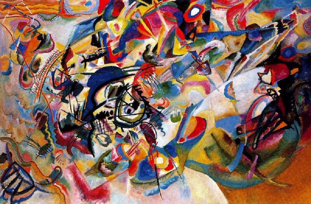
An example of style transfer A is a content image, B is output with style image in the bottom left corner
Architecture:
The neural style transfer paper uses feature maps generated by intermediate layers of VGG-19 network to generate the output image. This architecture takes style and content images as input and stores the features extracted by convolution layers of VGG network.

VGG-19 architecture
Content Loss:
To calculate the content cost, we apply the mean square difference between matrices generated by the content layer, when we pass the generated image and the original image. Let p and x be the original image and the image that is generated, and P and F are their respective feature representation in layer l. We then define the squared-error loss between the two feature representations

Style Loss:
To calculate the style cost, we will first calculate the gram matrix. The gram matrices calculation involves calculating the inner product between the vectorized feature maps of a particular layer. Here Gij (l) represents the inner product between vectorized features i,j of layer l.
Now to calculate the loss from a particular, we will find the mean square difference of gram matrices calculated from the feature vectors of the style image and the generated image. This then weighted to the layer weighing factor.
Let a and x be the original image and the generated image, and Al and Gl their respective style representation (gram matrices) in layer l. The contribution of layer l to the total loss is then:
Therefore, total style loss will be:
Total Loss
Total loss is the linear combination of style and content loss we defined above:
Where α and β are the weighting factors for content and style reconstruction, respectively.
Implementation in Tensorflow:
- First, we import the necessary module. In this post, we use TensorFlow v2 with Keras. We will also import VGG-19 model from tf.keras API.
Code:
Python3
# import numpy, tensorflow and matplotlibimport tensorflow as tfimport numpy as npimport matplotlib.pyplot as plt# import VGG 19 model and keras Model APIfrom tensorflow.python.keras.applications.vgg19 import VGG19, preprocess_inputfrom tensorflow.python.keras.preprocessing.image import load_img, img_to_arrayfrom tensorflow.python.keras.models import Model |
- Now, we import the content and style images and save them into our working directory.
Code:
Python3
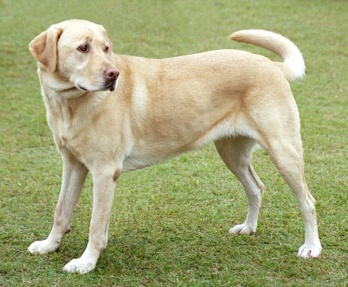
# Image Credits: Tensorflow Doccontent_path = tf.keras.utils.get_file('content.jpg', 'https://storage.googleapis.com/download.tensorflow.org/example_images/YellowLabradorLooking_new.jpg')style_path = tf.keras.utils.get_file('style.jpg', |
- Now, we initialize the VGG model with ImageNet weights, we will also remove the top layers and make it non-trainable.
Code:
Python3
# code# this function download the VGG model and initialise itmodel = VGG19( include_top=False, weights='imagenet')# set training to Falsemodel.trainable = False# Print details of different layersmodel.summary() |
Output:
Downloading data from https://storage.googleapis.com/tensorflow/keras-applications/vgg19/vgg19_weights_tf_dim_ordering_tf_kernels_notop.h5
80142336/80134624 [==============================] - 1s 0us/step
Model: "vgg19"
_________________________________________________________________
Layer (type)                 Output Shape              Param #
=================================================================
input_1 (InputLayer)         [(None, None, None, 3)]   0
_________________________________________________________________
block1_conv1 (Conv2D)        (None, None, None, 64)    1792
_________________________________________________________________
block1_conv2 (Conv2D)        (None, None, None, 64)    36928
_________________________________________________________________
block1_pool (MaxPooling2D)   (None, None, None, 64)    0
_________________________________________________________________
block2_conv1 (Conv2D)        (None, None, None, 128)   73856
_________________________________________________________________
block2_conv2 (Conv2D)        (None, None, None, 128)   147584
_________________________________________________________________
block2_pool (MaxPooling2D)   (None, None, None, 128)   0
_________________________________________________________________
block3_conv1 (Conv2D)        (None, None, None, 256)   295168
_________________________________________________________________
block3_conv2 (Conv2D)        (None, None, None, 256)   590080
_________________________________________________________________
block3_conv3 (Conv2D)        (None, None, None, 256)   590080
_________________________________________________________________
block3_conv4 (Conv2D)        (None, None, None, 256)   590080
_________________________________________________________________
block3_pool (MaxPooling2D)   (None, None, None, 256)   0
_________________________________________________________________
block4_conv1 (Conv2D)        (None, None, None, 512)   1180160
_________________________________________________________________
block4_conv2 (Conv2D)        (None, None, None, 512)   2359808
_________________________________________________________________
block4_conv3 (Conv2D)        (None, None, None, 512)   2359808
_________________________________________________________________
block4_conv4 (Conv2D)        (None, None, None, 512)   2359808
_________________________________________________________________
block4_pool (MaxPooling2D)   (None, None, None, 512)   0
_________________________________________________________________
block5_conv1 (Conv2D)        (None, None, None, 512)   2359808
_________________________________________________________________
block5_conv2 (Conv2D)        (None, None, None, 512)   2359808
_________________________________________________________________
block5_conv3 (Conv2D)        (None, None, None, 512)   2359808
_________________________________________________________________
block5_conv4 (Conv2D)        (None, None, None, 512)   2359808
_________________________________________________________________
block5_pool (MaxPooling2D)   (None, None, None, 512)   0
=================================================================
Total params: 20,024,384
Trainable params: 0
Non-trainable params: 20,024,384
________________________________________________________________
- Now, we load and process the image using Keras preprocess input in VGG 19. The expand_dims function adds a dimension to represent a number of images in the input. This preprocess_input function (used in VGG 19 ) converts the input RGB to BGR images and centre these values around 0 according to ImageNet data (no scaling).
Code:
Python3
# code to load and process imagedef load_and_process_image(image_path): img = load_img(image_path) # convert image to array img = img_to_array(img) img = preprocess_input(img) img = np.expand_dims(img, axis=0) return img |
- Now, we define the deprocess function that takes the input image and perform the inverse of preprocess_input function that we imported above. To display the unprocessed image, we also define a display function.
Code:
Python3
# codedef deprocess(img): # perform the inverse of the pre processing step img[:, :, 0] += 103.939 img[:, :, 1] += 116.779 img[:, :, 2] += 123.68 # convert RGB to BGR img = img[:, :, ::-1] img = np.clip(img, 0, 255).astype('uint8') return imgdef display_image(image): # remove one dimension if image has 4 dimension if len(image.shape) == 4: img = np.squeeze(image, axis=0) img = deprocess(img) plt.grid(False) plt.xticks([]) plt.yticks([]) plt.imshow(img) return |
- Now, we use the above function to display the style and content images
Code:
Python3
# load content imagecontent_img = load_and_process_image(content_path)display_image(content_img)# load style imagestyle_img = load_and_process_image(style_path)display_image(style_img) |
Output:

Content Image

Style Image
- Now, we define the content and style model using Keras.Model API. The content model takes the image as input and output the feature map from “block5_conv1” from the above VGG model.
Code:
Python3
# define content modelcontent_layer = 'block5_conv2'content_model = Model( inputs=model.input, outputs=model.get_layer(content_layer).output)content_model.summary() |
Output:
Model: "functional_9"
_________________________________________________________________
Layer (type)                 Output Shape              Param #
=================================================================
input_1 (InputLayer)         [(None, None, None, 3)]   0
_________________________________________________________________
block1_conv1 (Conv2D)        (None, None, None, 64)    1792
_________________________________________________________________
block1_conv2 (Conv2D)        (None, None, None, 64)    36928
_________________________________________________________________
block1_pool (MaxPooling2D)   (None, None, None, 64)    0
_________________________________________________________________
block2_conv1 (Conv2D)        (None, None, None, 128)   73856
_________________________________________________________________
block2_conv2 (Conv2D)        (None, None, None, 128)   147584
_________________________________________________________________
block2_pool (MaxPooling2D)   (None, None, None, 128)   0
_________________________________________________________________
block3_conv1 (Conv2D)        (None, None, None, 256)   295168
_________________________________________________________________
block3_conv2 (Conv2D)        (None, None, None, 256)   590080
_________________________________________________________________
block3_conv3 (Conv2D)        (None, None, None, 256)   590080
_________________________________________________________________
block3_conv4 (Conv2D)        (None, None, None, 256)   590080
_________________________________________________________________
block3_pool (MaxPooling2D)   (None, None, None, 256)   0
_________________________________________________________________
block4_conv1 (Conv2D)        (None, None, None, 512)   1180160
_________________________________________________________________
block4_conv2 (Conv2D)        (None, None, None, 512)   2359808
_________________________________________________________________
block4_conv3 (Conv2D)        (None, None, None, 512)   2359808
_________________________________________________________________
block4_conv4 (Conv2D)        (None, None, None, 512)   2359808
_________________________________________________________________
block4_pool (MaxPooling2D)   (None, None, None, 512)   0
_________________________________________________________________
block5_conv1 (Conv2D)        (None, None, None, 512)   2359808
_________________________________________________________________
block5_conv2 (Conv2D)        (None, None, None, 512)   2359808
=================================================================
Total params: 15,304,768
Trainable params: 0
Non-trainable params: 15,304,768
_________________________________________________________________
- Now, we define the content and style model using Keras.Model API. The style model takes an image as input and output the feature map from “block1_conv1, block3_conv1, and block5_conv2″ from the above VGG model.
Code:
Python3
# define style modelstyle_layers = [ 'block1_conv1', 'block3_conv1', 'block5_conv1']style_models = [Model(inputs=model.input, outputs=model.get_layer(layer).output) for layer in style_layers] |
- Now, we define the content loss function, it will take the feature map of generated and real images and calculate the mean square difference between them.
Code:
Python3
# Content lossdef content_loss(content, generated): a_C = content_model(content) loss = tf.reduce_mean(tf.square(a_C - a_G)) return loss |
- Now, we define the gram matrix and style loss function. This function also takes the real and generated images as the input of the model and calculates gram matrices of them before calculate the style loss weighted to different layers.
Code:
Python3
# gram matrixdef gram_matrix(A): channels = int(A.shape[-1]) a = tf.reshape(A, [-1, channels]) n = tf.shape(a)[0] gram = tf.matmul(a, a, transpose_a=True) return gram / tf.cast(n, tf.float32)weight_of_layer = 1. / len(style_models)# style lossdef style_cost(style, generated): J_style = 0 for style_model in style_models: a_S = style_model(style) a_G = style_model(generated) GS = gram_matrix(a_S) GG = gram_matrix(a_G) current_cost = tf.reduce_mean(tf.square(GS - GG)) J_style += current_cost * weight_of_layer return J_style |
- Now, we define our training function, we will train our model to 50 iterations. This model takes input images, the number of iterations as its argument.
Python3
# training functiongenerated_images = []def training_loop(content_path, style_path, iterations=50, a=10, b=1000): # load content and style images from their respective path content = load_and_process_image(content_path) style = load_and_process_image(style_path) generated = tf.Variable(content, dtype=tf.float32) opt = tf.keras.optimizers.Adam(learning_rate=7) best_cost = Inf best_image = None for i in range(iterations): % % time with tf.GradientTape() as tape: J_content = content_cost(content, generated) J_style = style_cost(style, generated) J_total = a * J_content + b * J_style grads = tape.gradient(J_total, generated) opt.apply_gradients([(grads, generated)]) if J_total < best_cost: best_cost = J_total best_image = generated.numpy() print("Iteration :{}".format(i)) print('Total Loss {:e}.'.format(J_total)) generated_images.append(generated.numpy()) return best_image |
- Now, we train our model using the training function we defined above.
Code:
Python3
# Train the model and get best imagefinal_img = training(content_path, style_path) |
Output:
CPU times: user 2 µs, sys: 1e+03 ns, total: 3 µs
Wall time: 6.2 µs
Iteration :0
Total Loss 5.133922e+11.
CPU times: user 2 µs, sys: 1e+03 ns, total: 3 µs
Wall time: 5.72 µs
Iteration :1
Total Loss 3.510511e+11.
CPU times: user 2 µs, sys: 1e+03 ns, total: 3 µs
Wall time: 6.68 µs
Iteration :2
Total Loss 2.069992e+11.
CPU times: user 3 µs, sys: 1e+03 ns, total: 4 µs
Wall time: 6.2 µs
Iteration :3
Total Loss 1.669609e+11.
CPU times: user 2 µs, sys: 1e+03 ns, total: 3 µs
Wall time: 6.44 µs
Iteration :4
Total Loss 1.575840e+11.
CPU times: user 2 µs, sys: 1e+03 ns, total: 3 µs
Wall time: 5.96 µs
Iteration :5
Total Loss 1.200623e+11.
CPU times: user 2 µs, sys: 1e+03 ns, total: 3 µs
Wall time: 5.96 µs
Iteration :6
Total Loss 8.824594e+10.
CPU times: user 2 µs, sys: 1e+03 ns, total: 3 µs
Wall time: 5.72 µs
Iteration :7
Total Loss 7.168546e+10.
CPU times: user 2 µs, sys: 1e+03 ns, total: 3 µs
Wall time: 5.48 µs
Iteration :8
Total Loss 6.207320e+10.
CPU times: user 3 µs, sys: 1e+03 ns, total: 4 µs
Wall time: 8.34 µs
Iteration :9
Total Loss 5.390836e+10.
CPU times: user 2 µs, sys: 1e+03 ns, total: 3 µs
Wall time: 6.2 µs
Iteration :10
Total Loss 4.735992e+10.
CPU times: user 2 µs, sys: 1e+03 ns, total: 3 µs
Wall time: 5.96 µs
Iteration :11
Total Loss 4.301782e+10.
CPU times: user 2 µs, sys: 1e+03 ns, total: 3 µs
Wall time: 6.2 µs
Iteration :12
Total Loss 3.912694e+10.
CPU times: user 2 µs, sys: 1e+03 ns, total: 3 µs
Wall time: 6.68 µs
Iteration :13
Total Loss 3.445185e+10.
CPU times: user 0 ns, sys: 3 µs, total: 3 µs
Wall time: 6.2 µs
Iteration :14
Total Loss 2.975165e+10.
CPU times: user 2 µs, sys: 0 ns, total: 2 µs
Wall time: 5.96 µs
Iteration :15
Total Loss 2.590984e+10.
CPU times: user 2 µs, sys: 1e+03 ns, total: 3 µs
Wall time: 20 µs
Iteration :16
Total Loss 2.302116e+10.
CPU times: user 2 µs, sys: 1e+03 ns, total: 3 µs
Wall time: 5.72 µs
Iteration :17
Total Loss 2.082643e+10.
CPU times: user 4 µs, sys: 1e+03 ns, total: 5 µs
Wall time: 8.34 µs
Iteration :18
Total Loss 1.906701e+10.
CPU times: user 2 µs, sys: 1e+03 ns, total: 3 µs
Wall time: 5.25 µs
Iteration :19
Total Loss 1.759801e+10.
CPU times: user 3 µs, sys: 1e+03 ns, total: 4 µs
Wall time: 6.2 µs
Iteration :20
Total Loss 1.635128e+10.
CPU times: user 2 µs, sys: 1e+03 ns, total: 3 µs
Wall time: 6.2 µs
Iteration :21
Total Loss 1.525327e+10.
CPU times: user 3 µs, sys: 1e+03 ns, total: 4 µs
Wall time: 5.96 µs
Iteration :22
Total Loss 1.418364e+10.
CPU times: user 4 µs, sys: 1 µs, total: 5 µs
Wall time: 9.06 µs
Iteration :23
Total Loss 1.306596e+10.
CPU times: user 2 µs, sys: 1e+03 ns, total: 3 µs
Wall time: 5.25 µs
Iteration :24
Total Loss 1.196509e+10.
CPU times: user 2 µs, sys: 1e+03 ns, total: 3 µs
Wall time: 5.96 µs
Iteration :25
Total Loss 1.102290e+10.
CPU times: user 2 µs, sys: 1e+03 ns, total: 3 µs
Wall time: 5.96 µs
Iteration :26
Total Loss 1.025539e+10.
CPU times: user 7 µs, sys: 3 µs, total: 10 µs
Wall time: 12.6 µs
Iteration :27
Total Loss 9.570500e+09.
CPU times: user 2 µs, sys: 1e+03 ns, total: 3 µs
Wall time: 5.72 µs
Iteration :28
Total Loss 8.917115e+09.
CPU times: user 2 µs, sys: 1e+03 ns, total: 3 µs
Wall time: 5.96 µs
Iteration :29
Total Loss 8.328761e+09.
CPU times: user 3 µs, sys: 1e+03 ns, total: 4 µs
Wall time: 9.54 µs
Iteration :30
Total Loss 7.840127e+09.
CPU times: user 2 µs, sys: 1e+03 ns, total: 3 µs
Wall time: 6.44 µs
Iteration :31
Total Loss 7.406647e+09.
CPU times: user 2 µs, sys: 1e+03 ns, total: 3 µs
Wall time: 8.34 µs
Iteration :32
Total Loss 6.967848e+09.
CPU times: user 2 µs, sys: 1e+03 ns, total: 3 µs
Wall time: 5.72 µs
Iteration :33
Total Loss 6.531650e+09.
CPU times: user 2 µs, sys: 1e+03 ns, total: 3 µs
Wall time: 5.72 µs
Iteration :34
Total Loss 6.136975e+09.
CPU times: user 2 µs, sys: 1 µs, total: 3 µs
Wall time: 5.96 µs
Iteration :35
Total Loss 5.788804e+09.
CPU times: user 2 µs, sys: 1e+03 ns, total: 3 µs
Wall time: 5.72 µs
Iteration :36
Total Loss 5.476942e+09.
CPU times: user 2 µs, sys: 1e+03 ns, total: 3 µs
Wall time: 6.2 µs
Iteration :37
Total Loss 5.204070e+09.
CPU times: user 3 µs, sys: 1 µs, total: 4 µs
Wall time: 6.2 µs
Iteration :38
Total Loss 4.954049e+09.
CPU times: user 2 µs, sys: 1e+03 ns, total: 3 µs
Wall time: 5.96 µs
Iteration :39
Total Loss 4.708641e+09.
CPU times: user 3 µs, sys: 2 µs, total: 5 µs
Wall time: 6.2 µs
Iteration :40
Total Loss 4.487677e+09.
CPU times: user 2 µs, sys: 1e+03 ns, total: 3 µs
Wall time: 5.96 µs
Iteration :41
Total Loss 4.296946e+09.
CPU times: user 2 µs, sys: 1e+03 ns, total: 3 µs
Wall time: 5.96 µs
Iteration :42
Total Loss 4.107909e+09.
CPU times: user 3 µs, sys: 1e+03 ns, total: 4 µs
Wall time: 6.44 µs
Iteration :43
Total Loss 3.918156e+09.
CPU times: user 3 µs, sys: 1e+03 ns, total: 4 µs
Wall time: 6.2 µs
Iteration :44
Total Loss 3.747263e+09.
CPU times: user 3 µs, sys: 1e+03 ns, total: 4 µs
Wall time: 8.34 µs
Iteration :45
Total Loss 3.595638e+09.
CPU times: user 2 µs, sys: 1e+03 ns, total: 3 µs
Wall time: 5.72 µs
Iteration :46
Total Loss 3.458928e+09.
CPU times: user 2 µs, sys: 1e+03 ns, total: 3 µs
Wall time: 6.2 µs
Iteration :47
Total Loss 3.331772e+09.
CPU times: user 4 µs, sys: 1e+03 ns, total: 5 µs
Wall time: 9.3 µs
Iteration :48
Total Loss 3.205911e+09.
CPU times: user 3 µs, sys: 1e+03 ns, total: 4 µs
Wall time: 5.96 µs
Iteration :49
Total Loss 3.089630e+09.
- In the final step, we plot the final and intermediate results.
Code:
Python3
# code to display best generated image and last 10 intermediate resultsplt.figure(figsize=(12, 12))for i in range(10): plt.subplot(4, 3, i + 1) display_image(generated_images[i+39])plt.show()# plot best resultdisplay_image(final_img) |
Output:

Last 10 Generated images

Best Generated image
References: