This article was published as a part of the Data Science Blogathon.
Overview
This article will see how to create a stacked sequence to sequence the LSTM model for time series forecasting in Keras/ TF 2.0.
Prerequisites: The reader should already be familiar with neural networks and, in particular, recurrent neural networks (RNNs). Also, knowledge of LSTM or GRU models is preferable. If you are not familiar with LSTM, I would prefer you to read LSTM- Long Short-Term Memory.
Introduction
In Sequence to Sequence Learning, an RNN model is trained to map an input sequence to an output sequence. The input and output need not necessarily be of the same length. The seq2seq model contains two RNNs, e.g., LSTMs. They can be treated as an encoder and decoder. The encoder part converts the given input sequence to a fixed-length vector, which acts as a summary of the input sequence.
This fixed-length vector is called the context vector. The context vector is given as input to the decoder and the final encoder state as an initial decoder state to predict the output sequence. Sequence to Sequence learning is used in language translation, speech recognition, time series
forecasting, etc.
We will use the sequence to sequence learning for time series forecasting. We can use this architecture to easily make a multistep forecast. we will add two layers, a repeat vector layer and time distributed dense layer in the architecture.
A repeat vector layer is used to repeat the context vector we get from the encoder to pass it as an input to the decoder. We will repeat it for n-steps ( n is the no of future steps you want to forecast). The output received from the decoder with respect to each time step is mixed. The time distributed densely will apply a fully connected dense layer on each time step and separates the output for each timestep. The time distributed densely is a wrapper that allows applying a layer to every temporal slice of an input.
We will stack additional layers on the encoder part and the decoder part of the sequence to sequence model. By stacking LSTM’s, it may increase the ability of our model to understand more complex representation of our time-series data in hidden layers, by capturing information at different levels.
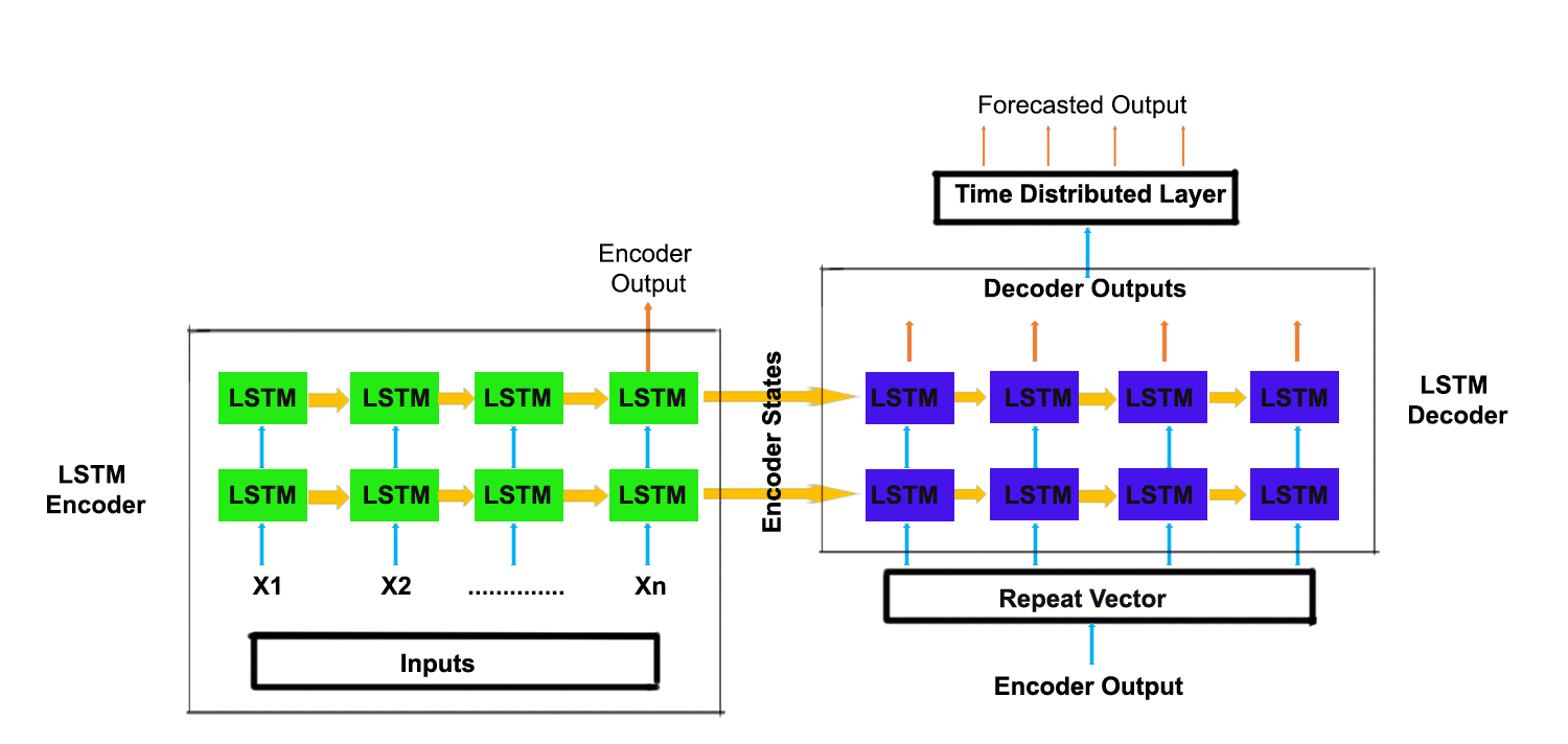
Table of contents
What is the role of LSTM Layer in Keras?
The LSTM (Long Short-Term Memory) layer in Keras plays a vital role in modeling sequential data. It is designed to handle the challenges of capturing and processing long-term dependencies within sequential input. The layer contains memory cells that can retain information over extended periods, enabling the network to learn patterns and relationships in sequences such as time series or natural language data.
LSTM layers excel in mitigating the vanishing gradient problem associated with traditional RNNs. This problem occurs when gradients diminish during backpropagation, limiting the network’s ability to learn long-term dependencies. LSTMs address this by utilizing a gating mechanism that regulates the flow of information into and out of memory cells. This allows them to selectively retain or discard information, facilitating the modeling of complex sequential patterns.
By incorporating LSTM layers into a neural network, the model gains the capability to capture and understand dependencies across multiple time steps or positions in the input sequence. This makes LSTMs particularly useful in various applications, including machine translation, sentiment analysis, speech recognition, and time series forecasting, where understanding and modeling the temporal relationships is crucial for accurate predictions.
Code of Keras LSTM Layer to Predict Electric Power Consumption
The data used is Individual household electric power consumption. You can download the dataset from this link.
Importing Libraries
import pandas as pd
import numpy as np
from sklearn.preprocessing import MinMaxScaler
import matplotlib.pyplot as plt
import tensorflow as tf
import os
Now load the dataset into a pandas data frame.
df=pd.read_csv(r'household_power_consumption.txt', sep=';', header=0, low_memory=False, infer_datetime_format=True, parse_dates={'datetime':[0,1]}, index_col=['datetime'])
df.head()

Imputing Null Values
df = df.replace('?', np.nan)
df.isnull().sum()
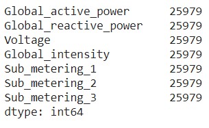
Now we will create a function that will impute missing values by replacing them with values on their previous day.
def fill_missing(values):
    one_day = 60*24
    for row in range(df.shape[0]):
        for col in range(df.shape[1]):
            if np.isnan(values[row][col]):
                values[row,col] = values[row-one_day,col]
df = df.astype('float32')
fill_missing(df.values)
df.isnull().sum()
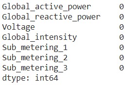
Downsampling of Data from minutes to Days
There are more than 2 lakh observations recorded. Let’s make the data simpler by downsampling them from the frequency of minutes to days.
daily_df = df.resample('D').sum()
daily_df.head()

Train – Test Split
After downsampling, the number of instances is 1442. We will split the dataset into train and test data in a 75% and 25% ratio of the instances. (0.75 * 1442 = 1081)
train_df,test_df = daily_df[1:1081], daily_df[1081:]
Scaling the values
All the columns in the data frame are on a different scale. Now we will scale the values to -1 to 1 for faster training of the models.
train = train_df
scalers={}
for i in train_df.columns:
    scaler = MinMaxScaler(feature_range=(-1,1))
    s_s = scaler.fit_transform(train[i].values.reshape(-1,1))
    s_s=np.reshape(s_s,len(s_s))
    scalers['scaler_'+ i] = scaler
    train[i]=s_s
test = test_df
for i in train_df.columns:
    scaler = scalers['scaler_'+i]
    s_s = scaler.transform(test[i].values.reshape(-1,1))
    s_s=np.reshape(s_s,len(s_s))
    scalers['scaler_'+i] = scaler
    test[i]=s_s
Converting the series to samples
Now we will make a function that will use a sliding window approach to transform our series into samples of input past observations and output future observations to use supervised learning algorithms.
def split_series(series, n_past, n_future):
  #
  # n_past ==> no of past observations
  #
  # n_future ==> no of future observations
  #
  X, y = list(), list()
  for window_start in range(len(series)):
    past_end = window_start + n_past
    future_end = past_end + n_future
    if future_end > len(series):
      break
    # slicing the past and future parts of the window
    past, future = series[window_start:past_end, :], series[past_end:future_end, :]
    X.append(past)
    y.append(future)
  return np.array(X), np.array(y)
For this case, let’s assume that given the past 10 days observation, we need to forecast the next 5 days observations.
n_past = 10
n_future = 5
n_features = 7
Now convert both the train and test data into samples using the split_series function.
X_train, y_train = split_series(train.values,n_past, n_future)
X_train = X_train.reshape((X_train.shape[0], X_train.shape[1],n_features))
y_train = y_train.reshape((y_train.shape[0], y_train.shape[1], n_features))
X_test, y_test = split_series(test.values,n_past, n_future)
X_test = X_test.reshape((X_test.shape[0], X_test.shape[1],n_features))
y_test = y_test.reshape((y_test.shape[0], y_test.shape[1], n_features))
Model Architecture
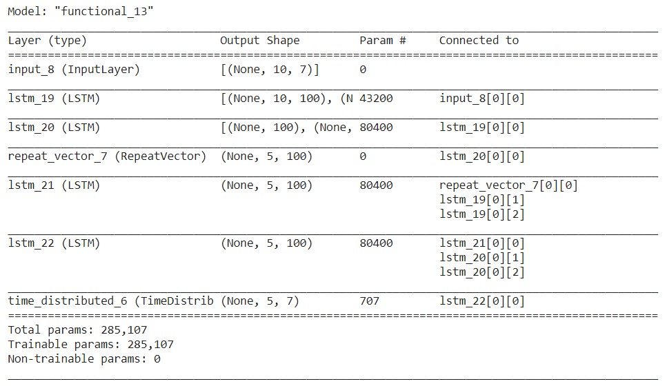
Now we will create two models in the below-mentioned architecture.
E1D1 ==> Sequence to Sequence Model with one encoder layer and one decoder layer.
# E1D1
# n_features ==> no of features at each timestep in the data.
#
encoder_inputs = tf.keras.layers.Input(shape=(n_past, n_features))
encoder_l1 = tf.keras.layers.LSTM(100, return_state=True)
encoder_outputs1 = encoder_l1(encoder_inputs)

encoder_states1 = encoder_outputs1[1:]

#
decoder_inputs = tf.keras.layers.RepeatVector(n_future)(encoder_outputs1[0])

#
decoder_l1 = tf.keras.layers.LSTM(100, return_sequences=True)(decoder_inputs,initial_state = encoder_states1)
decoder_outputs1 = tf.keras.layers.TimeDistributed(tf.keras.layers.Dense(n_features))(decoder_l1)

#
model_e1d1 = tf.keras.models.Model(encoder_inputs,decoder_outputs1)

#
model_e1d1.summary()
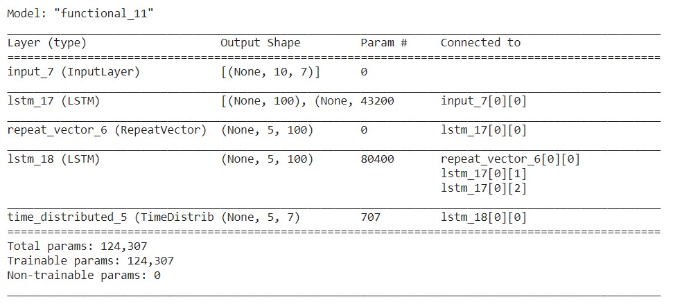
E2D2 ==> Sequence to Sequence Model with two encoder layers and two decoder layers.
# E2D2
# n_features ==> no of features at each timestep in the data.
#
encoder_inputs = tf.keras.layers.Input(shape=(n_past, n_features))
encoder_l1 = tf.keras.layers.LSTM(100,return_sequences = True, return_state=True)
encoder_outputs1 = encoder_l1(encoder_inputs)
encoder_states1 = encoder_outputs1[1:]
encoder_l2 = tf.keras.layers.LSTM(100, return_state=True)
encoder_outputs2 = encoder_l2(encoder_outputs1[0])
encoder_states2 = encoder_outputs2[1:]
#
decoder_inputs = tf.keras.layers.RepeatVector(n_future)(encoder_outputs2[0])
#
decoder_l1 = tf.keras.layers.LSTM(100, return_sequences=True)(decoder_inputs,initial_state = encoder_states1)
decoder_l2 = tf.keras.layers.LSTM(100, return_sequences=True)(decoder_l1,initial_state = encoder_states2)
decoder_outputs2 = tf.keras.layers.TimeDistributed(tf.keras.layers.Dense(n_features))(decoder_l2)
#
model_e2d2 = tf.keras.models.Model(encoder_inputs,decoder_outputs2)
#
model_e2d2.summary()
Training the models
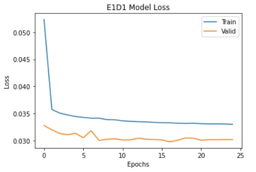
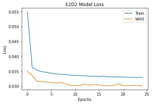
I have used Adam optimizer and Huber loss as the loss function. Let’s compile and run the model.
reduce_lr = tf.keras.callbacks.LearningRateScheduler(lambda x: 1e-3 * 0.90 ** x)
model_e1d1.compile(optimizer=tf.keras.optimizers.Adam(), loss=tf.keras.losses.Huber())
history_e1d1=model_e1d1.fit(X_train,y_train,epochs=25,validation_data=(X_test,y_test),batch_size=32,verbose=0,callbacks=[reduce_lr])
model_e2d2.compile(optimizer=tf.keras.optimizers.Adam(), loss=tf.keras.losses.Huber())
history_e2d2=model_e2d2.fit(X_train,y_train,epochs=25,validation_data=(X_test,y_test),batch_size=32,verbose=0,callbacks=[reduce_lr])
Prediction on test samples
pred_e1d1=model_e1d1.predict(X_test)
pred_e2d2=model_e2d2.predict(X_test)
Inverse Scaling of the predicted values
Now we will convert the predictions to their original scale.
for index,i in enumerate(train_df.columns):
    scaler = scalers['scaler_'+i]
    pred1_e1d1[:,:,index]=scaler.inverse_transform(pred1_e1d1[:,:,index])
    pred_e1d1[:,:,index]=scaler.inverse_transform(pred_e1d1[:,:,index])
    pred1_e2d2[:,:,index]=scaler.inverse_transform(pred1_e2d2[:,:,index])
    pred_e2d2[:,:,index]=scaler.inverse_transform(pred_e2d2[:,:,index])
    y_train[:,:,index]=scaler.inverse_transform(y_train[:,:,index])
    y_test[:,:,index]=scaler.inverse_transform(y_test[:,:,index])
Checking Error
Now we will calculate the mean absolute error of all observations.
from sklearn.metrics import mean_absolute_error
for index,i in enumerate(train_df.columns):
  print(i)
  for j in range(1,6):
    print("Day ",j,":")
    print("MAE-E1D1 : ",mean_absolute_error(y_test[:,j-1,index],pred1_e1d1[:,j-1,index]),end=", ")
    print("MAE-E2D2 : ",mean_absolute_error(y_test[:,j-1,index],pred1_e2d2[:,j-1,index]))
  print()
  print()
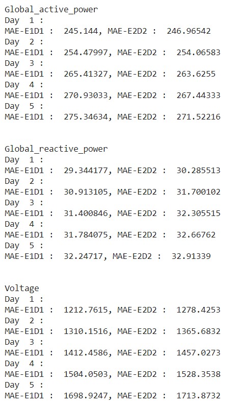
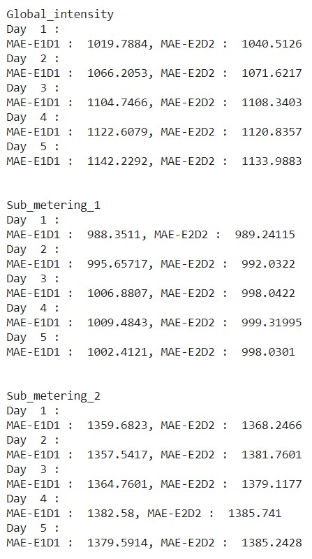
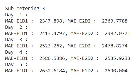
From the above output, we can observe that, in some cases, the E2D2 model has performed better than the E1D1 model with less error. Training different models with a different number of stacked layers and creating an ensemble model also performs well.
Note: The results vary with respect to the dataset. If we stack more layers, it may also lead to overfitting. So the number of layers to be stacked acts as a hyperparameter.
Frequently Asked Questions
A. In Keras, LSTM (Long Short-Term Memory) is a type of recurrent neural network (RNN) layer. LSTM networks are designed to capture and process sequential information, such as time series or natural language data, by mitigating the vanishing gradient problem in traditional RNNs. LSTM layers provide memory cells that retain information over long periods, making them effective for modeling temporal dependencies in sequential data.
A. To use LSTM layers in Keras, you can follow these steps:
1. Import the necessary modules from Keras.
2. Create a sequential model or functional model.
3. Add an LSTM layer using LSTM() and specify the desired number of units and other parameters.
4. Optionally, add additional LSTM layers or other types of layers.
5. Compile and train the model using appropriate data and settings.
6. Evaluate or make predictions using the trained model.
A. LSTMs (Long Short-Term Memory) are preferred over CNNs (Convolutional Neural Networks) in certain scenarios because LSTMs excel at capturing sequential dependencies in data, such as time series or natural language data, while CNNs are better suited for extracting spatial features from fixed-size inputs like images. LSTMs’ ability to retain long-term information and model temporal dependencies makes them suitable for tasks involving sequential data analysis.
Conclusion
Congratulations, you have learned how to implement multivariate multi-step time series forecasting using TF 2.0 / Keras. This is my first attempt at writing a blog. So please share your opinion in the comments section below.
Thanks for reading.
References:
1. https://machinelearningmastery.com/how-to-develop-lstm-models-for-time-series-forecasting/
2. https://blog.keras.io/a-ten-minute-introduction-to-sequence-to-sequence-learning-in-keras.html
3. https://archive.ics.uci.edu/ml/datasets/Individual+household+electric+power+consumption


