This article was published as a part of the Data Science Blogathon
Overview
This article will discuss building a system that can detect malaria from cell images. The plan will be created in the form of a web application that can make it easier for users and even make it easier for developers who make webs.
Algorithm for Classification Malaria Cell Image Using Deep Learning
The first thing to do after getting the dataset is to perform an image data generator, which rescales the image and then sets the target size (150, 150) and then divides the data into training and test data. For the classification of malaria cell images, preprocessing does not take a long time. After preprocessing, we create a deep learning architecture using a Convolutional Neural Network. In this section, we have to define the number of convolutions that we will operate along with the activation function, kernel size, filters, and the number of dense layers of how many neurons to set. Then to compile the model, we need loss, optimizer, and metrics. Next, to fit the model, we must set the number of epochs, validation step, step per epoch, and verbose.
Load Data
Because the data processing uses Google Colab and the dataset source is from Kaggle, the dataset taken from Kaggle is saved to google drive using the code below:
! pip install -q kaggle
from google.colab import files
files.upload()
! mkdir ~/.kaggle
! cp kaggle.json ~/.kaggle/
import os
os.chdir('drive/MyDrive/.../')
!kaggle datasets download -d iarunava/cell-images-for-detecting-malaria #download dataset from kaggle
After downloading the dataset, we have to extract the file because the downloaded file is in .zip format.
import os
# Complete path to storage location of the .zip file of data
zip_path = '/content/drive/MyDrive/Kaggle/cell-images-for-detecting-malaria.zip'
# Check current directory (be sure you're in the directory where Colab operates: '/content')
os.getcwd()
# Copy the .zip file into the present directory
!cp '{zip_path}' .
# Unzip quietly
!unzip -q 'cell-images-for-detecting-malaria.zip'
# View the unzipped contents in the virtual machine
os.listdir()
Preprocessing
As explained in the algorithm subsection above, we first do the preprocessing as follows.
from tensorflow.keras.preprocessing.image import ImageDataGenerator
#image data generataor
datagen = ImageDataGenerator(
                    rescale=1./255,
                    validation_split = 0.2)
train_generator = datagen.flow_from_directory(
    path_dir,
    target_size=(150,150),
    shuffle=True,
    subset='training'
)
validation_generator = datagen.flow_from_directory(
    path_dir,
    target_size=(150,150),
    subset='validation'
)
Build Model
- Define a model which takes (None, 150, 150, 3) input. Stack 4 convolutional layers with kernel size (3, 3) with a growing number of filters (32, 64, 128, 128). Add 2×2 pooling layer after every 2 convolutional layers (conv-conv-pool scheme). Add a dense layer with 512 neurons and a second dense layer with two neurons for classes.
import tensorflow as tf
#Activation function: relu and sigmoid
model = tf.keras.models.Sequential([
    #first_convolution
    tf.keras.layers.Conv2D(32, (3,3), activation='relu', input_shape=(150, 150, 3)),
    tf.keras.layers.MaxPooling2D(2, 2),
    #second_convolution
    tf.keras.layers.Conv2D(64, (3,3), activation='relu'),
    tf.keras.layers.MaxPooling2D(2,2),
    #third_convolution
    tf.keras.layers.Conv2D(128, (3,3), activation='relu'),
    tf.keras.layers.MaxPooling2D(2,2),
    #fourth_convolution
    tf.keras.layers.Conv2D(128, (3,3), activation='relu'),
    tf.keras.layers.MaxPooling2D(2,2),
    tf.keras.layers.Flatten(),
    tf.keras.layers.Dropout(0.5),
    # 512 neuron hidden layer
    tf.keras.layers.Dense(512, activation='relu'),
    tf.keras.layers.Dense(2, activation='sigmoid')
])
- Compile model, with adam optimizer and binary cross-entropy for loss function:
model.compile(loss='binary_crossentropy',
              optimizer=tf.optimizers.Adam(),
              metrics=['accuracy'])
- Fit Model , with 25 steps_per_epoch, 20 epochs, 5 validation_steps, and 2 verbose:
model.fit(
      train_generator,
      steps_per_epoch=25,
      epochs=20,
      validation_data=validation_generator,
      validation_steps=5,
      verbose=2)
Epoch 1/20
25/25 - 49s - loss: 0.6959 - accuracy: 0.5175 - val_loss: 0.7033 - val_accuracy: 0.4313
Epoch 2/20
25/25 - 39s - loss: 0.6328 - accuracy: 0.6562 - val_loss: 0.7640 - val_accuracy: 0.7750
Epoch 3/20
25/25 - 39s - loss: 0.5175 - accuracy: 0.7875 - val_loss: 0.3806 - val_accuracy: 0.8750
Epoch 4/20
25/25 - 39s - loss: 0.3837 - accuracy: 0.8850 - val_loss: 0.3086 - val_accuracy: 0.9312
Epoch 5/20
25/25 - 39s - loss: 0.2298 - accuracy: 0.9225 - val_loss: 0.1345 - val_accuracy: 0.9500
Epoch 6/20
25/25 - 39s - loss: 0.2213 - accuracy: 0.9262 - val_loss: 0.2110 - val_accuracy: 0.9438
Epoch 7/20
25/25 - 39s - loss: 0.1808 - accuracy: 0.9350 - val_loss: 0.1000 - val_accuracy: 0.9563
Epoch 8/20
25/25 - 39s - loss: 0.1673 - accuracy: 0.9337 - val_loss: 0.3180 - val_accuracy: 0.9062
Epoch 9/20
25/25 - 38s - loss: 0.1937 - accuracy: 0.9375 - val_loss: 0.1052 - val_accuracy: 0.9750
Epoch 10/20
25/25 - 39s - loss: 0.1674 - accuracy: 0.9438 - val_loss: 0.1593 - val_accuracy: 0.9250
Epoch 11/20
25/25 - 39s - loss: 0.2266 - accuracy: 0.9450 - val_loss: 0.1387 - val_accuracy: 0.9375
Epoch 12/20
25/25 - 39s - loss: 0.1866 - accuracy: 0.9425 - val_loss: 0.2648 - val_accuracy: 0.9125
Epoch 13/20
25/25 - 38s - loss: 0.1623 - accuracy: 0.9525 - val_loss: 0.2226 - val_accuracy: 0.9187
Epoch 14/20
25/25 - 38s - loss: 0.1764 - accuracy: 0.9500 - val_loss: 0.1876 - val_accuracy: 0.9375
Epoch 15/20
25/25 - 39s - loss: 0.1775 - accuracy: 0.9500 - val_loss: 0.1868 - val_accuracy: 0.9250
Epoch 16/20
25/25 - 41s - loss: 0.1780 - accuracy: 0.9438 - val_loss: 0.1737 - val_accuracy: 0.9312
Epoch 17/20
25/25 - 38s - loss: 0.1750 - accuracy: 0.9525 - val_loss: 0.1473 - val_accuracy: 0.9438
Epoch 18/20
25/25 - 38s - loss: 0.1859 - accuracy: 0.9438 - val_loss: 0.1117 - val_accuracy: 0.9625
Epoch 19/20
25/25 - 38s - loss: 0.1270 - accuracy: 0.9550 - val_loss: 0.1153 - val_accuracy: 0.9438
Epoch 20/20
25/25 - 38s - loss: 0.1630 - accuracy: 0.9525 - val_loss: 0.2125 - val_accuracy: 0.9125
- Based on the fit model results, we can see the accuracy of the training and validate its accuracy. The training accuracy is 0.9525 or 95.25%, and the validation accuracy is 91.25%.
- Save Model and Predict:
model.save("malaria_cell.h5") #the model is saved with the name malaria_cell.h5
Confusion Matrix to see test results
In the last part, we will look at testing the data using the confusion matrix. This will show how much test data we have and how much data was misclassified by the system.
import tensorflow as tf
from sklearn.metrics import confusion_matrix
import seaborn as sns
import numpy as np
import matplotlib.pyplot as plt
pred = model.predict(validation_generator)
y_pred = np.argmax(pred, axis=1)
y_true = np.argmax(pred, axis=1)
print('confusion matrix')
print(confusion_matrix(y_true, y_pred))
    #confusion matrix
f, ax = plt.subplots(figsize=(8,5))
sns.heatmap(confusion_matrix(y_true, y_pred), annot=True, fmt=".0f", ax=ax)
plt.xlabel("y_pred")
plt.ylabel("y_true")
plt.show()
Output:
confusion matrix
[[2798    0]
 [   0 2712]]
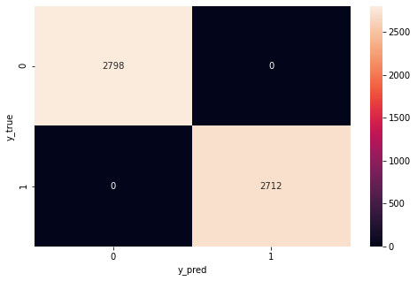
Or it can be visualized like the following image.

Note: 0 label is Parasitized and 1 label is Uninfected.
This model achieves 95.25% accuracy during training and 91.25% on validation or testing.
GUI for Malaria Cell Image Classification
The system that was made previously only came to conducting training and testing on the Convolutional Neural Network architectural model that was created. The accuracy of the training and testing produced is also good. This can be seen from the Confusion Matrix displayed at the end of the test. But the system created still has shortcomings. Yes, Graphical User Interface. The system that has been made is quite suitable where this system has successfully carried out the test with an accuracy of 0.9125or 91.25%. However, this system can only be run by a Machine Learning Engineer who implements the calculations to perform classification/prediction into a program. Of course, the system created is not only for use by Machine Learning Engineers. Remember, the goal is to help health workers make it easier to diagnose. This means that this system must be run or operated by the user (in this case, the user in question is a health worker) to detect or classify which cell images are infected with malaria and which are not infected. For this reason, we need to create a GUI so that it is easier for health workers or users to operate the system created.
Streamlit
Streamlit turns data scripts into shareable web apps in minutes. All in Python. All for free. No front-end experience is required. That’s Streamlit. We will create web apps using Streamlit to make it easier for users to operate the malaria cell image classification system we created using deep learning techniques. With Streamlit, it’s not only users who find it easier to operate the system; programmers or developers also find it easier to create web apps. With streamlit, developers also don’t need experience developing a web or working as a front-end developer. Streamlit is trusted by more than 50% of Fortune 50 companies, such as IBM, UBER, TESLA, WALMART, Intel, Apple, and many more. Streamlit is also used in the world’s top data science groups. Streamlit Compatible with libraries in python such as matplotlib, bokeh, plotly, scikit-learn, pandas, numpy, hard, tensorflow, opencv, and even more, with Streamlit Components
Get Started in Under a Minute
Streamlit’s open-source app framework is a breeze to get started with. It’s just a matter of:
pip install streamlit
Building Web Applications
Import library. Required libraries:
Streamlit. Streamlit is the main library needed to create web apps.
Tensorflow. Why Tensorflow? First, tensorFlow is an end-to-end open source platform for machine learning. It has a comprehensive, flexible ecosystem of tools, libraries and community resources that lets researchers push the state-of-the-art in ML and developers easily build and deploy ML powered applications. Second, The deep learning model we created using the hard library from tensorflow. We have also saved the built model, and this model will be loaded in this web application.
Numpy. Numpy is very necessary to process the arrangement of images that we load.
PIL. PIL or Pillow is Python Imaging Library. This library is very useful for loading images from operating system and performing operations on loaded images (image processing).
import streamlit as st #we can call this library as st in the code that we will create.
import tensorflow as tf #we can call this library as tf in the code.
import numpy as np #we can call this library as np in the code.
from PIL import Image, ImageOps #we can call this library for load images and performing operations on load images.
Creat webpage header:
st.write("""
# Malaria Cell Classification
"""
)
Create a sidebar for uploading files with the name or title on the sidebar ‘Upload Cell Image’ and type png:
upload_file = st.sidebar.file_uploader("Upload Cell Images", type="png")
Create a button on the sidebar to make predictions:
Generate_pred=st.sidebar.button("Predict")
Loads the created CNN model:
model=tf.keras.models.load_model('malaria_cell.h5') #The model created, saved under the name malaria_cell.h5.
Create functions for import and prediction/classification of images:
def import_n_pred(image_data, model):
    size = (150,150)
    image = ImageOps.fit(image_data, size, Image.ANTIALIAS)
    img = np.asarray(image)
    reshape=img[np.newaxis,...]
    pred = model.predict(reshape)
    return pred
In the function created above, we set the image size (150, 150) then perform operations on the image by calling the ImageOps mode. In operations using ImageOps, we also add ANTIALIAS. When ANTIALIAS was initially added, it was the only high-quality filter based on convolutions. Next, create an image into a numpy array and reshape the array, and perform predictions or classifications by calling the model using the model.predict syntax from tensorflow. The return is the pred variable, which is the prediction result.
Displays the results when the user performs the action pressing the predict button in the sidebar:
if Generate_pred:
    image=Image.open(upload_file)
    with st.beta_expander('Cell Image', expanded = True):
        st.image(image, use_column_width=True)
    pred=import_n_pred(image, model)
    labels = ['Parasitized', 'Uninfected']
    st.title("Prediction of image is {}".format(labels[np.argmax(pred)]))
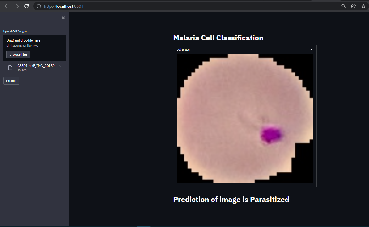
The simple explanation, if the user presses the predict button, then he also act an action on the Generate pred variable and will perform actions such as, the system will open the image file to be uploaded, then it will call the import function and the prediction is made and perform the prediction then it will show the label ‘Parasitized’ ‘ or ‘Uninfected’ of the image.
Full Code of GUI
This is the entire coding of the codes above:
"""
@author: Abdiel W. Goni
"""
import streamlit as st
import tensorflow as tf
import numpy as np
from PIL import Image, ImageOps
st.write("""
          # Malaria Cell Classification
          """
          )
upload_file = st.sidebar.file_uploader("Upload Cell Images", type="png")
Generate_pred=st.sidebar.button("Predict")
model=tf.keras.models.load_model('malaria_cell.h5')
def import_n_pred(image_data, model):
    size = (150,150)
    image = ImageOps.fit(image_data, size, Image.ANTIALIAS)
    img = np.asarray(image)
    reshape=img[np.newaxis,...]
    pred = model.predict(reshape)
    return pred
if Generate_pred:
    image=Image.open(upload_file)
    with st.beta_expander('Cell Image', expanded = True):
        st.image(image, use_column_width=True)
    pred=import_n_pred(image, model)
    labels = ['Parasitized', 'Uninfected']
    st.title("Prediction of image is {}".format(labels[np.argmax(pred)]))
To run this code, type: streamlit run /your path and .py name in your command prompt.
GUI Display
Before uploading files and making predictions:
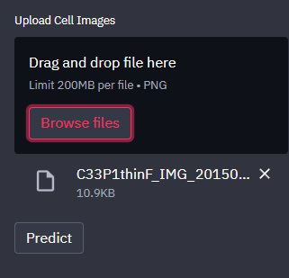
Browse File:

Prediction Result:

Conclusion
Malaria cell image classification uses deep learning faster than most traditional machine learning techniques. The final result of GUI creation is very satisfactory, where the system prediction results or sort of cell images are not in doubt. Display GUI is very user-friendly. With Streamlit, we can save time creating web apps and don’t need front-end capabilities. That’s it. See you at another time.
The media shown in this article is not owned by Analytics Vidhya and are used at the Author’s discretion.


