Introduction
If you have spent some time in machine learning and data science, you would have definitely come across imbalanced class distribution. This is a scenario where the number of observations belonging to one class is significantly lower than those belonging to the other classes.
This problem is predominant in scenarios where anomaly detection is crucial like electricity pilferage, fraudulent transactions in banks, identification of rare diseases, etc. In this situation, the predictive model developed using conventional machine learning algorithms could be biased and inaccurate.
This happens because Machine Learning Algorithms are usually designed to improve accuracy by reducing the error. Thus, they do not take into account the class distribution / proportion or balance of classes.
This guide describes various approaches for solving such class imbalance problems using various sampling techniques. We also weigh each technique for its pros and cons. Finally, I reveal an approach using which you can create a balanced class distribution and apply ensemble learning technique designed especially for this purpose.
Table of contents
Challenges faced with imbalanced data
One of the main challenges faced by the utility industry today is electricity theft. Electricity theft is the third largest form of theft worldwide. Utility companies are increasingly turning towards advanced analytics and machine learning algorithms to identify consumption patterns that indicate theft.
However, one of the biggest stumbling blocks is the humongous data and its distribution. Fraudulent transactions are significantly lower than normal healthy transactions i.e. accounting it to around 1-2 % of the total number of observations. The ask is to improve identification of the rare minority class as opposed to achieving higher overall accuracy.
Machine Learning algorithms tend to produce unsatisfactory classifiers when faced with imbalanced datasets. For any imbalanced data set, if the event to be predicted belongs to the minority class and the event rate is less than 5%, it is usually referred to as a rare event.
Example of imbalanced data
Let’s understand this with the help of an example.
Ex: In an utilities fraud detection data set you have the following data:
Total Observations = 1000
Fraudulent Observations = 20
Non Fraudulent Observations = 980
Event Rate= 2 %
The main question faced during data analysis is – How to get a balanced dataset by getting a decent number of samples for these anomalies given the rare occurrence for some them?
Challenges with standard Machine learning techniques
The conventional model evaluation methods do not accurately measure model performance when faced with imbalanced datasets.
Standard classifier algorithms like Decision Tree and Logistic Regression have a bias towards classes which have number of instances. They tend to only predict the majority class data. The features of the minority class are treated as noise and are often ignored. Thus, there is a high probability of misclassification of the minority class as compared to the majority class.
Evaluation of a classification algorithm performance is measured by the Confusion Matrix which contains information about the actual and the predicted class.
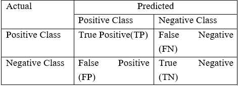
Accuracy of a model = (TP+TN) / (TP+FN+FP+TN)
However, while working in an imbalanced domain accuracy is not an appropriate measure to evaluate model performance. For eg: A classifier which achieves an accuracy of 98 % with an event rate of 2 % is not accurate, if it classifies all instances as the majority class. And eliminates the 2 % minority class observations as noise.
Examples of imbalanced data
Thus, to sum it up, while trying to resolve specific business challenges with imbalanced data sets, the classifiers produced by standard machine learning algorithms might not give accurate results. Apart from fraudulent transactions, other examples of a common business problem with imbalanced dataset are:
- Datasets to identify customer churn where a vast majority of customers will continue using the service. Specifically, Telecommunication companies where Churn Rate is lower than 2 %.
- Data sets to identify rare diseases in medical diagnostics etc.
- Natural Disaster like Earthquakes
Dataset used
In this article, we will illustrate the various techniques to train a model to perform well against highly imbalanced datasets. And accurately predict rare events using the following fraud detection dataset:
Total Observations = 1000
Fraudulent Observations =20
Non-Fraudulent Observations = 980
Event Rate= 2 %
Fraud Indicator = 0 for Non-Fraud Instances
Fraud Indicator = 1 for Fraud
Approach to handling Imbalanced Data
2.1 Data Level approach: Resampling Techniques
Dealing with imbalanced datasets entails strategies such as improving classification algorithms or balancing classes in the training data (data preprocessing) before providing the data as input to the machine learning algorithm. The later technique is preferred as it has wider application.
The main objective of balancing classes is to either increasing the frequency of the minority class or decreasing the frequency of the majority class. This is done in order to obtain approximately the same number of instances for both the classes. Let us look at a few resampling techniques:
2.1.1 Random Under-Sampling
Random Undersampling aims to balance class distribution by randomly eliminating majority class examples. This is done until the majority and minority class instances are balanced out.
Total Observations = 1000
Fraudulent Observations =20
Non Fraudulent Observations = 980
Event Rate= 2 %
In this case we are taking 10 % samples without replacement from Non Fraud instances. And combining them with Fraud instances.
Non Fraudulent Observations after random under sampling = 10 % of 980 =98
Total Observations after combining them with Fraudulent observations = 20+98=118
Event Rate for the new dataset after under sampling = 20/118 = 17%
- Advantages
- It can help improve run time and storage problems by reducing the number of training data samples when the training data set is huge.
- Disadvantages
- It can discard potentially useful information which could be important for building rule classifiers.
- The sample chosen by random under sampling may be a biased sample. And it will not be an accurate representative of the population. Thereby, resulting in inaccurate results with the actual test data set.
2.1.2 Random Over-Sampling
Over-Sampling increases the number of instances in the minority class by randomly replicating them in order to present a higher representation of the minority class in the sample.
Total Observations = 1000
Fraudulent Observations =20
Non Fraudulent Observations = 980
Event Rate= 2 %
In this case we are replicating 20 fraud observations 20 times.
Non Fraudulent Observations =980
Fraudulent Observations after replicating the minority class observations= 400
Total Observations in the new data set after oversampling=1380
Event Rate for the new data set after under sampling= 400/1380 = 29 %
- Advantages
- Unlike under sampling this method leads to no information loss.
- Outperforms under sampling
- Disadvantages
- It increases the likelihood of overfitting since it replicates the minority class events.
2.1.3 Cluster-Based Over Sampling
In this case, the K-means clustering algorithm is independently applied to minority and majority class instances. This is to identify clusters in the dataset. Subsequently, each cluster is oversampled such that all clusters of the same class have an equal number of instances and all classes have the same size.
Total Observations = 1000
Fraudulent Observations =20
Non Fraudulent Observations = 980
Event Rate= 2 %
- Majority Class Clusters
- Cluster 1: 150 Observations
- Cluster 2: 120 Observations
- Cluster 3: 230 observations
- Cluster 4: 200 observations
- Cluster 5: 150 observations
- Cluster 6: 130 observations
- Minority Class Clusters
- Cluster 1: 8 Observations
- Cluster 2: 12 Observations
After oversampling of each cluster, all clusters of the same class contain the same number of observations.
- Majority Class Clusters
- Cluster 1: 170 Observations
- Cluster 2: 170 Observations
- Cluster 3: 170 observations
- Cluster 4: 170 observations
- Cluster 5: 170 observations
- Cluster 6: 170 observations
- Minority Class Clusters
- Cluster 1: 250 Observations
- Cluster 2: 250 Observations
Event Rate post cluster based oversampling sampling = 500/ (1020+500) = 33 %
- Advantages
- This clustering technique helps overcome the challenge between class imbalance. Where the number of examples representing positive class differs from the number of examples representing a negative class.
- Also, overcome challenges within class imbalance, where a class is composed of different sub clusters. And each sub cluster does not contain the same number of examples.
- Disadvantages
- The main drawback of this algorithm, like most oversampling techniques is the possibility of over-fitting the training data.
2.1.4 Informed Over Sampling: Synthetic Minority Over-sampling Technique for imbalanced data
This technique is followed to avoid overfitting which occurs when exact replicas of minority instances are added to the main dataset. A subset of data is taken from the minority class as an example and then new synthetic similar instances are created. These synthetic instances are then added to the original dataset. The new dataset is used as a sample to train the classification models.
Total Observations = 1000
Fraudulent Observations = 20
Non Fraudulent Observations = 980
Event Rate = 2 %
A sample of 15 instances is taken from the minority class and similar synthetic instances are generated 20 times
Post generation of synthetic instances, the following data set is created
Minority Class (Fraudulent Observations) = 300
Majority Class (Non-Fraudulent Observations) = 980
Event rate= 300/1280 = 23.4 %
- Advantages
- Mitigates the problem of overfitting caused by random oversampling as synthetic examples are generated rather than replication of instances
- No loss of useful information
- Disadvantages
- While generating synthetic examples SMOTE does not take into consideration neighboring examples from other classes. This can result in increase in overlapping of classes and can introduce additional noise
- SMOTE is not very effective for high dimensional data
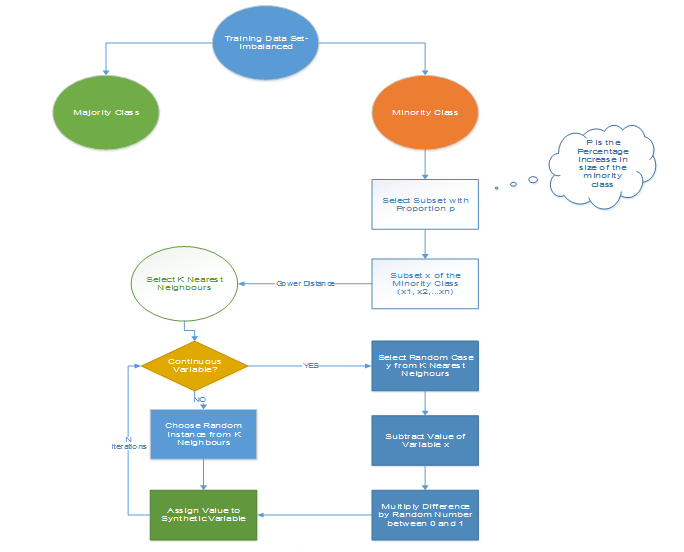
**N is the number of attributes
Figure 1: Synthetic Minority Oversampling Algorithm
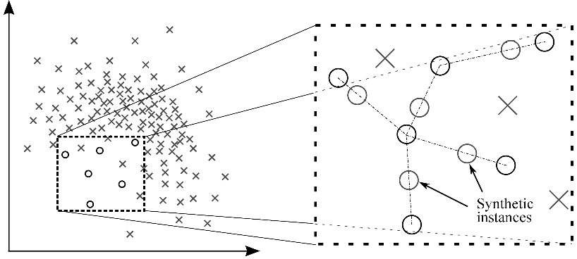
Figure 2: Generation of Synthetic Instances with the help of SMOTE
2.1.5 Modified synthetic minority oversampling technique (MSMOTE) for imbalanced data
It is a modified version of SMOTE. SMOTE does not consider the underlying distribution of the minority class and latent noises in the dataset. To improve the performance of SMOTE a modified method MSMOTE is used.
This algorithm classifies the samples of minority classes into 3 distinct groups – Security/Safe samples, Border samples, and latent nose samples. This is done by calculating the distances among samples of the minority class and samples of the training data.
Security samples are those data points which can improve the performance of a classifier. While on the other hand, noise are the data points which can reduce the performance of the classifier. The ones which are difficult to categorize into any of the two are classified as border samples.
While the basic flow of MSOMTE is the same as that of SMOTE (discussed in the previous section). In MSMOTE the strategy of selecting nearest neighbors is different from SMOTE. The algorithm randomly selects a data point from the k nearest neighbors for the security sample, selects the nearest neighbor from the border samples and does nothing for latent noise.
2.2 Algorithmic Ensemble Techniques
The above section, deals with handling imbalanced data by resampling original data to provide balanced classes. In this section, we are going to look at an alternate approach i.e. Modifying existing classification algorithms to make them appropriate for imbalanced data sets.
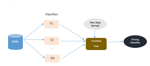
The main objective of ensemble methodology is to improve the performance of single classifiers. The approach involves constructing several two stage classifiers from the original data and then aggregate their predictions.
Figure 3: Approach to Ensemble based Methodologies
2.2.1. Bagging Based techniques for imbalanced data
Bagging is an abbreviation of Bootstrap Aggregating. The conventional bagging algorithm involves generating ‘n’ different bootstrap training samples with replacement. And training the algorithm on each bootstrapped algorithm separately and then aggregating the predictions at the end.
Bagging is used for reducing Overfitting in order to create strong learners for generating accurate predictions. Unlike boosting, bagging allows replacement in the bootstrapped sample.
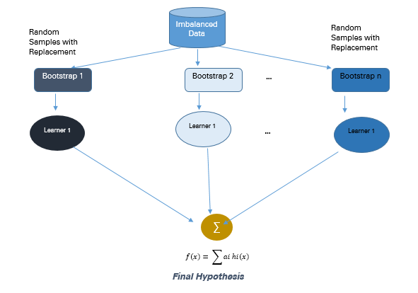
Figure 4: Approach to Bagging Methodology
Total Observations = 1000
Fraudulent Observations =20
Non Fraudulent Observations = 980
Event Rate= 2 %
There are 10 bootstrapped samples chosen from the population with replacement. Each sample contains 200 observations. And each sample is different from the original dataset but resembles the dataset in distribution & variability.
The machine learning algorithms like logistic regression, neural networks, decision tree are fitted to each bootstrapped sample of 200 observations. And the Classifiers c1, c2…c10 are aggregated to produce a compound classifier. This ensemble methodology produces a stronger compound classifier since it combines the results of individual classifiers to come up with an improved one.
- Advantages
- Improves stability & accuracy of machine learning algorithms
- Reduces variance
- Overcomes overfitting
- Improved misclassification rate of the bagged classifier
- In noisy data environments bagging outperforms boosting
- Disadvantages
- Bagging works only if the base classifiers are not bad to begin with. Bagging bad classifiers can further degrade performance
2.2.2. Boosting-Based techniques for imbalanced data
Boosting is an ensemble technique to combine weak learners to create a strong learner that can make accurate predictions. Boosting starts out with a base classifier / weak classifier that is prepared on the training data.
What are base learners / weak classifiers?
The base learners / Classifiers are weak learners i.e. the prediction accuracy is only slightly better than average. A classifier learning algorithm is said to be weak when small changes in data induce big changes in the classification model.
In the next iteration, the new classifier focuses on or places more weight to those cases which were incorrectly classified in the last round.
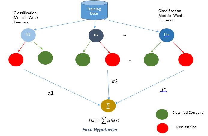
Figure 5: Approach to Boosting Methodologies
2.2.2.1. Adaptive Boosting- Ada Boost techniques for imbalanced data
Ada Boost is the first original boosting technique which creates a highly accurate prediction rule by combining many weak and inaccurate rules. Each classifier is serially trained with the goal of correctly classifying examples in every round that were incorrectly classified in the previous round.
For a learned classifier to make strong predictions it should follow the following three conditions:
- The rules should be simple
- Classifier should have been trained on sufficient number of training examples
- The Classifier should have low training error for the training instances
Each of the weak hypothesis has an accuracy slightly better than random guessing i.e. Error Term € (t) should be slightly more than ½-β where β >0. This is the fundamental assumption of this boosting algorithm which can produce a final hypothesis with a small error
After each round, it gives more focus to examples that are harder to classify. The quantity of focus is measured by a weight, which initially is equal for all instances. After each iteration, the weights of misclassified instances are increased and the weights of correctly classified instances are decreased.
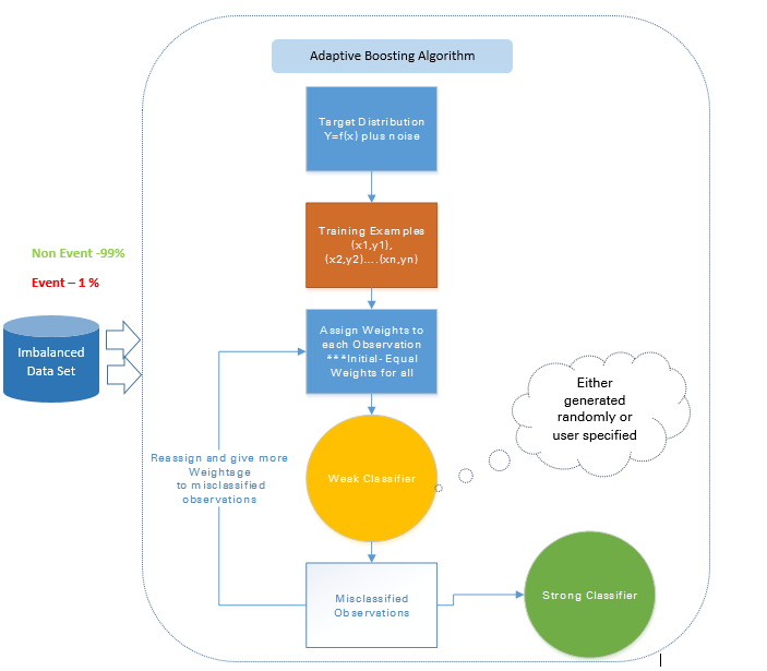
Figure 6: Approach to Adaptive Boosting
For example in a data set containing 1000 observations out of which 20 are labelled fraudulent. Equal weights W1 are assigned to all observations and the base classifier accurately classifies 400 observations.
Weight of each of the 600 misclassified observations is increased to w2 and weight of each of the correctly classified observations is reduced to w3.
In each iteration, these updated weighted observations are fed to the weak classifier to improve its performance. This process continues till the misclassification rate significantly decreases thereby resulting in a strong classifier.
- Advantages
- Very Simple to implement
- Good generalization- suited for any kind of classification problem ü Not prone to overfitting
- Disadvantages
- Sensitive to noisy data and outliers
2.2.2.2 Gradient Tree Boosting techniques for imbalanced data
In Gradient Boosting many models are trained sequentially. It is a numerical optimization algorithm where each model minimizes the loss function, y = ax+b+e, using the Gradient Descent Method.
Decision Trees are used as weak learners in Gradient Boosting.
While both Adaboost and Gradient Boosting work on weak learners / classifiers. And try to boost them into a strong learner, there are some fundamental differences in the two methodologies. Adaboost either requires the users to specify a set of weak learners or randomly generates the weak learners before the actual learning process. The weight of each learner is adjusted at every step depending on whether it predicts a sample correctly.
On the other hand, Gradient Boosting builds the first learner on the training dataset to predict the samples, calculates the loss (Difference between real value and output of the first learner). And use this loss to build an improved learner in the second stage.
At every step, the residual of the loss function is calculated using the Gradient Descent Method and the new residual becomes a target variable for the subsequent iteration.
Gradient Boosting can be done using the Gradient Boosting Node in SAS Miner and GBM package in R
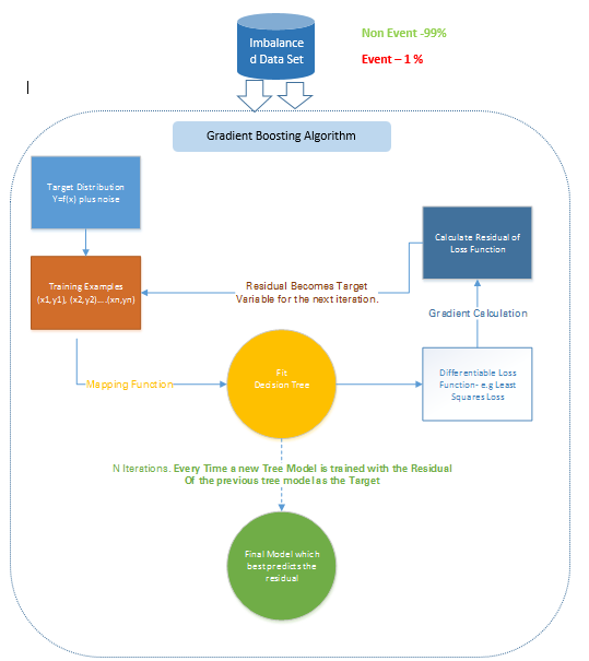
Figure 7: Approach to Gradient Boosting
For example: In a training data set containing 1000 observations out of which 20 are labelled fraudulent an initial base classifier. Target Variable Fraud =1 for fraudulent transactions and Fraud=0 for not fraud transactions.
For eg: Decision tree is fitted which accurately classifying only 5 observations as Fraudulent observations. A differentiable loss function is calculated based on the difference between the actual output and the predicted output of this step. The residual of the loss function is the target variable (F1) for the next iteration.
Similarly, this algorithm internally calculates the loss function, updates the target at every stage and comes up with an improved classifier as compared to the initial classifier.
- Disadvantages
- Gradient Boosted trees are harder to fit than random forests
- Gradient Boosting Algorithms generally have 3 parameters which can be fine-tuned, Shrinkage parameter, depth of the tree, the number of trees. Proper training of each of these parameters is needed for a good fit. If parameters are not tuned correctly it may result in over-fitting.
2.2.2.3 XG Boost techniques for imbalanced data
XGBoost (Extreme Gradient Boosting) is an advanced and more efficient implementation of Gradient Boosting Algorithm discussed in the previous section.
Advantages over Other Boosting Techniques
- It is 10 times faster than the normal Gradient Boosting as it implements parallel processing. It is highly flexible as users can define custom optimization objectives and evaluation criteria, has an inbuilt mechanism to handle missing values.
- Unlike gradient boosting which stops splitting a node as soon as it encounters a negative loss, XG Boost splits up to the maximum depth specified and prunes the tree backward and removes splits beyond which there is an only negative loss.
Extreme gradient boosting can be done using the XGBoost package in R and Python
Illustrative Example on dealing with imbalanced data
3.1. Data Description
The illustrative telecom churn dataset has 47241 client records with each record containing information about 27 key predictor variables.

The data structure of the rare event data set is shown below post missing value removal, outlier treatment and dimension reduction.

Download the Dataset from here: Sample Dataset
3.2 Description of Methodologies
The unbalanced dataset is balanced using Synthetic Minority oversampling technique (SMOTE) which attempts to balance the data set by creating synthetic instances. And train the balanced data set using Gradient Boosting Algorithm as illustrated by the R codes in the next section
R Codes
#Load Data
rareevent_boost <- read.table("D:/Upasana/RareEvent/churn.txt",sep="|", header=TRUE)
dmy<-dummyVars("~.",data=rareevent_boost)
rareeventTrsf<-data.frame(predict(dmy,newdata= rareevent_boost))
set.seed(10)
sub <- sample(nrow(rareeventTrsf), floor(nrow(rareeventTrsf) * 0.9))
sub1 <- sample(nrow(rareeventTrsf), floor(nrow(rareeventTrsf) * 0.1))
training <- rareeventTrsf [sub, ]
testing <- rareeventTrsf [-sub, ]
training_sub<- rareeventTrsf [sub1, ]
tables(training_sub)
head(training_sub)
#for unbalanced data set#
install.packages("unbalanced")
library(unbalanced)
data(ubIonosphere)
n<-ncol(rareevent_boost)
output<- rareevent_boost $CHURN_FLAG
output<-as.factor(output)
input<- rareevent_boost [ ,-n]
View(input)
#Balance the Dataset using ubSMOTE#
data<-ubBalance(X= input, Y=output, type="ubSMOTE", percOver=300, percUnder=150, verbose=TRUE
View(data)
#Balanced Data#
balancedData<-cbind(data$X,data$Y)
View(balancedData)
table(balancedData$CHURN_FLAG)
#Write the balanced data to be used to train the model#
write.table(balancedData,"D:/ Upasana/RareEvent /balancedData.txt", sep="\t", row.names=FALSE)
#Build Boosting tree Model#
repalceNAsWithMean <- function(x) {replace(x, is.na(x), mean(x[!is.na(x)]))}
training <- repalceNAsWithMean(training)
testing <- repalceNAsWithMean(testing)
#Resampling Technique#
View(train_set)
fitcontrol<-trainControl(method="repeatedcv",number=10,repeats=1,verbose=FALSE)
gbmfit<-train(CHURN_FLAG~.,data=balancedData,method="gbm",verbose=FALSE)
#Score test Data#
testing$score_Y=predict(gbmfit,newdata=testing,type="prob")[,2]
testing$score_Y=ifelse(testing$score_Y>0.5,1,0)
head(testing,n=10)
write.table(testing,"D:/ Upasana/RareEvent /testing.txt", sep="\t", row.names=FALSE)
pred_GBM<-prediction(testing$score_Y,testing$CHURN_FLAG)
#Model Performance#
model_perf_GBM <- performance(pred_GBM, "tpr", "fpr")
model_perf_GBM1 <- performance(pred_GBM, "tpr", "fpr")
model_perf_GBM
pred_GBM1<-as.data.frame(model_perf_GBM)
auc.tmp_GBM <- performance(pred_GBM,"auc")
AUC_GBM <- as.numeric([email protected])
auc.tmp_GBM
Results
This approach of balancing the data set with SMOTE and training a gradient boosting algorithm on the balanced set significantly impacts the accuracy of the predictive model. By increasing its lift by around 20% and precision/hit ratio by 3-4 times as compared to normal analytical modeling techniques like logistic regression and decision trees.
Frequently Asked Questions
A. A classic example of class imbalance is email spam classification, where the majority of emails are legitimate (non-spam), and only a small fraction are spam messages. This imbalance makes it challenging for machine learning models to accurately detect spam, as they might favor the majority class (non-spam) and have lower sensitivity to the minority class (spam).
A. Class imbalance refers to a situation in a dataset where the distribution of classes or categories is highly uneven. In such cases, one or more classes have significantly fewer instances compared to others. This imbalance can pose challenges in machine learning, as algorithms may struggle to properly learn and make accurate predictions for the minority class, leading to biased results and reduced performance.
Conclusion
When faced with imbalanced data sets there is no one stop solution to improve the accuracy of the prediction model. One may need to try out multiple methods to figure out the best-suited sampling techniques for the dataset. In most cases, synthetic techniques like SMOTE and MSMOTE will outperform the conventional oversampling and undersampling methods.
For better results, one can use synthetic sampling methods like SMOTE and MSMOTE along with advanced boosting methods like Gradient boosting and XG Boost.
One of the advanced bagging techniques commonly used to counter the imbalanced dataset problem is SMOTE bagging. It follows an entirely different approach from conventional bagging to create each Bag/Bootstrap. It generates the positive instances by the SMOTE Algorithm by setting a SMOTE resampling rate in each iteration. The set of negative instances is bootstrapped in each iteration.
Depending on the characteristics of the imbalanced data set, the most effective techniques will vary. Relevant evaluation parameters should be considered during the model comparison.
While comparing multiple prediction models built through an exhaustive combination of the above-mentioned techniques Lift & Area under the ROC Curve will be instrumental in determining which model is superior to the others.
If you have any questions or doubts, feel free to drop them in the comments below.
References
- Dmitry Pavlov, Alexey Gorodilov, Cliff Brunk “BagBoo: A Scalable Hybrid Bagging-theBoosting Model”.2010
- Fithria Siti Hanifah , Hari Wijayanto , Anang Kurnia “SMOTE Bagging Algorithm for Imbalanced Data Set in Logistic Regression Analysis”. Applied Mathematical Sciences, Vol. 9, 2015
- Lina Guzman, DIRECTV “Data sampling improvement by developing SMOTE technique in SAS” .Paper 3483-2015
- Mikel Galar, Alberto Fern´andez, Edurne Barrenechea, Humberto Bustince and Francisco Herrera “A Review on Ensembles for the Class Imbalance Problem: Bagging-, Boosting-, and Hybrid-Based Approaches “ .2011 IEEE
About the Author

Upasana holds a Post Graduate diploma in Management from Indian Institute of Management, Indore. She is currently working as a Consultant in the Data & Analytics Practice of KPMG. She has around 3.5 + years of work experience and has worked in multiple advanced analytics and data science engagements spanning industries like Telecom, utilities, banking , manufacturing. She has worked extensively on SAS, Data Management & Advanced Analytics, R, Tableau, Oracle and SQL.


