


Introduction
So far we’ve seen three feature selection techniques- Missing Value Ratio, Low Variance Filter, and Backward Feature Elimination. In this article, we’re going to learn one more technique used for feature selection and that is Forward Feature Selection. It is basically the opposite of Backward feature elimination. Let’s look at how!
Note: If you are more interested in learning concepts in an Audio-Visual format, We have this entire article explained in the video below. If not, you may continue reading.
We’ll use the same example of fitness level prediction based on the three independent variables-
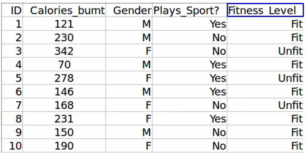
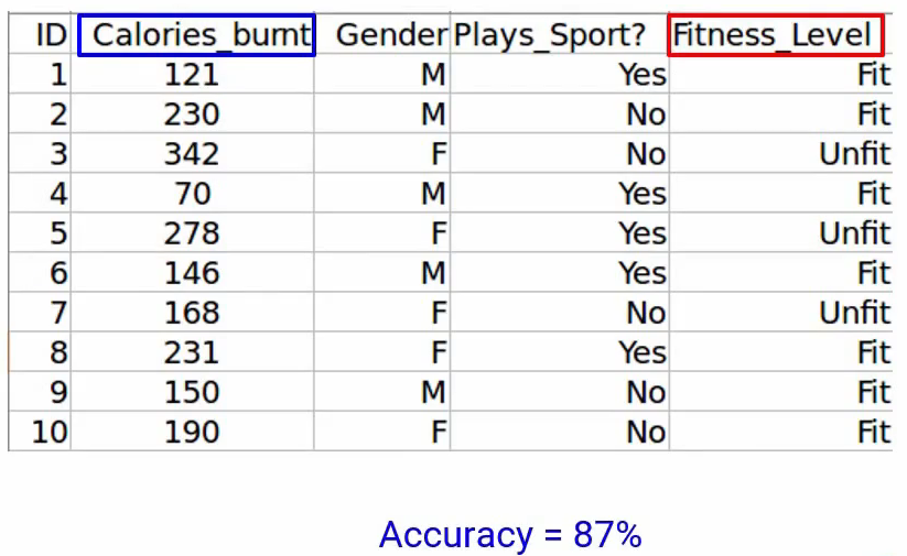
So the first step in Forward Feature Selection is to train n models using each feature individually and checking the performance. So if you have three independent variables, we will train three models using each of these three features individually. Let’s say we trained the model using the Calories_Burnt feature and the target variable, Fitness_Level and we’ve got an accuracy of 87%-
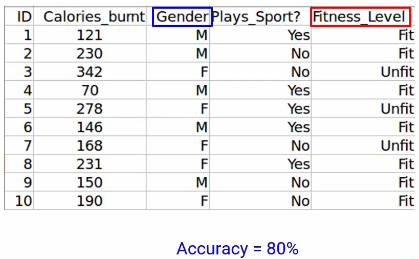
Next, we’ll train the model using the Gender feature, and we get an accuracy of 80%-
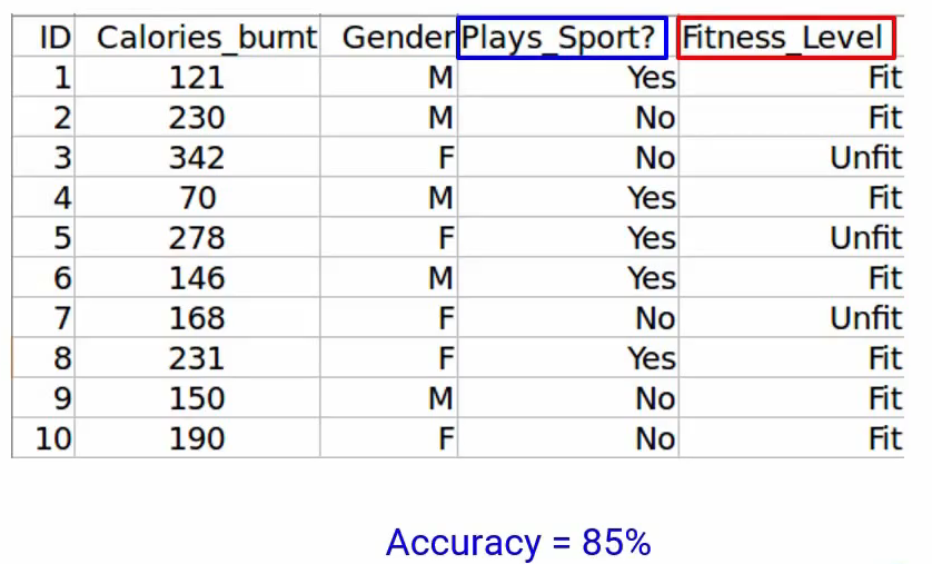
And similarly, the Plays_sport variable gives us an accuracy of 85%–
Now we will choose the variable, which gives us the best performance. When you look at this table-
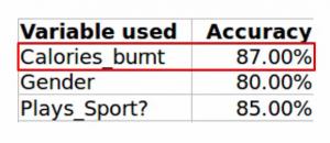
as you can see Calories_Burnt alone gives an accuracy of 87% and Gender give 80% and the Plays_Sport variable gives 85%. When we compare these values, of course, Calories_Burnt produced the best result. And hence, we will select this variable.
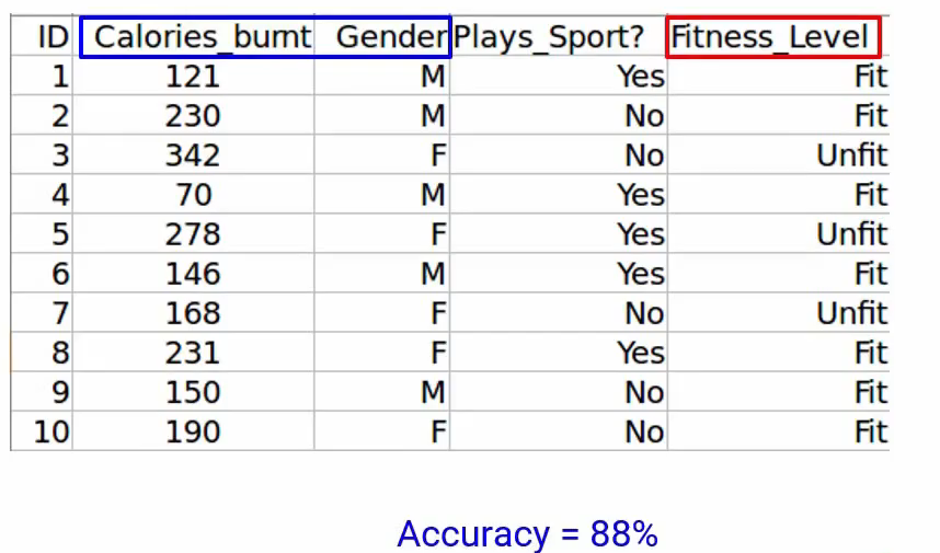
Next, we will repeat this process and add one variable at a time. So of course we’ll keep the Calories_Burnt variable and keep adding one variable. So let’s take Gender here and using this we get an accuracy of 88%-
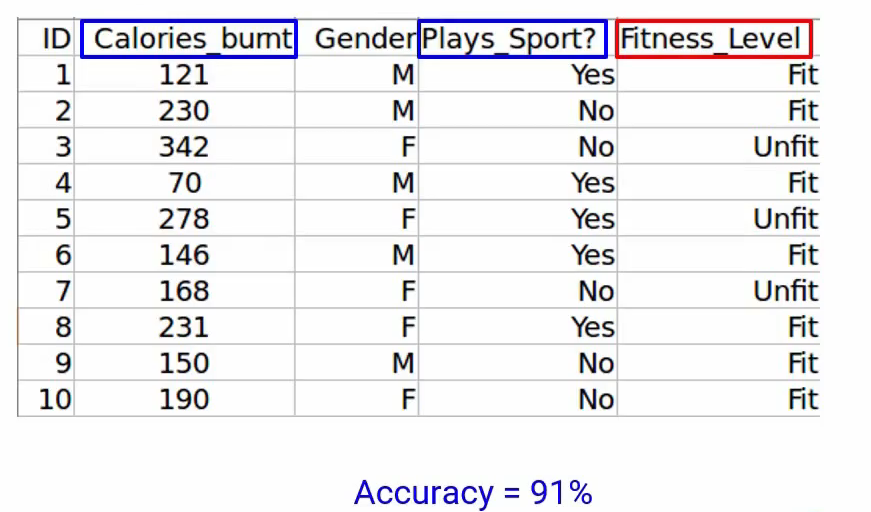
When you take Plays_Sport along with Calories_Burnt, we get an accuracy of 91%. A variable that produces the highest improvement will be retained. That intuitively makes sense. As you can see, Plays_Sport gives us a better accuracy when we combined it with the Calories_Burnt. Hence we will retain that and select it in our model. We will repeat the entire process until there is no significant improvement in the model’s performance.
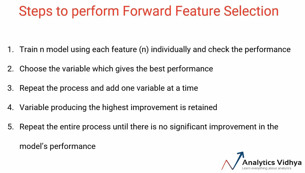
Summary:
Implementation of Forward Feature Selection
Now let’s see how we can implement Forward Feature Selection and get a practical understanding of this method. So first import the Pandas library as pd-
#importing the libraries
import pandas as pd
Then read the dataset and print the first five observations using the data.head() function-
#reading the file
data = pd.read_csv('forward_feature_selection.csv')

# first 5 rows of the data
data.head()
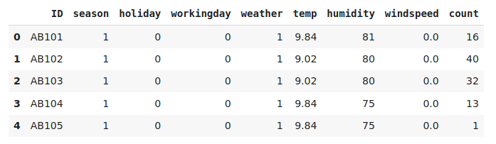
We have “the Count” target variable and the other independent variables. Let’s check out the shape of our data-
#shape of the data
data.shape
It comes out to be 12,980 observations again, and 9 columns of variables. Perfect! Are there any missing values?
# checking missing values in the data
data.isnull().sum()
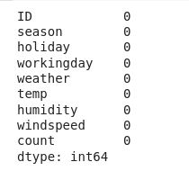
Nope! There are none, we can move on. Now again, since we are training a model on a dataset, we need to explicitly define the target variable and the independent variables. X will be the independent variables here after dropping the ID variable. And we’ll take Y as the target variable “Count”-
# creating the training data
X = data.drop(['ID', 'count'], axis=1)
y = data['count']
Let me look at the shapes of both-
X.shape, y.shape
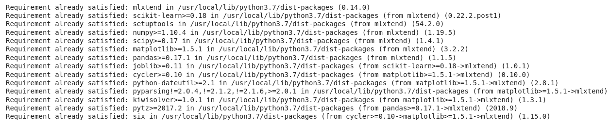
Perfect! Next, we will install the mlxtend library, we already did this in the backward elimination method. If you don’t have it installed, you can go ahead and do this step-
!pip install mlxtend
Now from the recently installed mlxtend we’ll import SequentialFeatureSelector and from the sklearn library, we’ll import LinearReggression since we are working on a regression problem where we have to predict the count of bikes rented.
# importing the models

from mlxtend.feature_selection import SequentialFeatureSelector as sfs
from sklearn.linear_model import LinearRegression
Let’s go ahead and train our model. Here, similar to what we did in the backward elimination technique, we first call the Linear Regression model. And then we define the Feature Selector Model-
# calling the linear regression model

lreg = LinearRegression()
sfs1 = sfs(lreg, k_features=4, forward=True, verbose=2, scoring='neg_mean_squared_error')
In the Feature Selector Model let me quickly recap what these different parameters are. The first parameter is the model name, lreg, which is basically our linear regression model.
k_features tells us how many features should be selected. We’ve passed 4 so the model will train until 4 features are selected.
Now here’s the difference between implementing the Backward Elimination Method and the Forward Feature Selection method, the parameter forward will be set to True. This means training the forward feature selection model. We set it as False during the backward feature elimination technique.
Next, verbose = 2 will allow us to bring the model summary at each iteration.
And finally, since it is a regression model scoring based on the mean squared error metric, we will set scoring = ‘neg_mean_squared_error’
Let’s go ahead and fit the model. Here we go!
sfs1 = sfs1.fit(X, y)
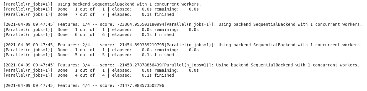
We can see that the model was trained until four features were selected. Let me print the feature names-
feat_names = list(sfs1.k_feature_names_)
print(feat_names)
It seems pretty familiar, holiday, working day, temp and humidity. These were the exact same features that were selected in a backward elimination method. Awesome right?
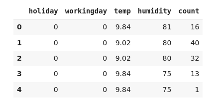
But keep in mind that this might not be the case when you’re working on a different problem. This is not a rule. It just so happened, occurred in our particular data. So let’s put these features into a new data frame and print the first five observations-
# creating a new dataframe using the above variables and adding the target variable
new_data = data[feat_names]
new_data['count'] = data['count']

# first five rows of the new data
new_data.head()
Perfect! Lastly, let’s have a look at the shape of both datasets-
# shape of new and original data
new_data.shape, data.shape
A quick look at the shape of the two datasets does confirm that we have indeed selected four variables from our original data.
You’ve done it again and that was fun!
End Notes
This is all for now with respect to Forward Feature Elimination.
If you are looking to kick start your Data Science Journey and want every topic under one roof, your search stops here. Check out Analytics Vidhya’s Certified AI & ML BlackBelt Plus Program
If you have any queries let me know in the comment section!
I am a data lover and I love to extract and understand the hidden patterns in the data. I want to learn and grow in the field of Machine Learning and Data Science.