This article was published as a part of the Data Science Blogathon.
Introduction
Feedforward Neural Networks, also known as Deep feedforward Networks or Multi-layer Perceptrons, are the focus of this article. For example, Convolutional and Recurrent Neural Networks (which are used extensively in computer vision applications) are based on these networks. We’ll do our best to grasp the key ideas in an engaging and hands-on manner without having to delve too deeply into mathematics.
Search engines, machine translation, and mobile applications all rely on deep learning technologies. It works by stimulating the human brain in terms of identifying and creating patterns from various types of input.
A feedforward neural network is a key component of this fantastic technology since it aids software developers with pattern recognition and classification, non-linear regression, and function approximation.
What is Feedforward Neural Network?
A feedforward neural network is a type of artificial neural network in which nodes’ connections do not form a loop.
Often referred to as a multi-layered network of neurons, feedforward neural networks are so named because all information flows in a forward manner only.
The data enters the input nodes, travels through the hidden layers, and eventually exits the output nodes. The network is devoid of links that would allow the information exiting the output node to be sent back into the network.
The purpose of feedforward neural networks is to approximate functions.
Here’s how it works
There is a classifier using the formula y = f* (x).
This assigns the value of input x to the category y.
The feedfоrwаrd netwоrk will mар y = f (x; θ). It then memorizes the value of θ that most closely approximates the function.
As shown in the Google Photos app, a feedforward neural network serves as the foundation for object detection in photos.
A Feedforward Neural Network’s Layers
The following are the components of a feedforward neural network:
Layer of input
It contains the neurons that receive input. The data is subsequently passed on to the next tier. The input layer’s total number of neurons is equal to the number of variables in the dataset.
Hidden layer
This is the intermediate layer, which is concealed between the input and output layers. This layer has a large number of neurons that perform alterations on the inputs. They then communicate with the output layer.
Output layer
It is the last layer and is depending on the model’s construction. Additionally, the output layer is the expected feature, as you are aware of the desired outcome.
Neurons weights
Weights are used to describe the strength of a connection between neurons. The range of a weight’s value is from 0 to 1.
Cost Function in Feedforward Neural Network
The cost function is an important factor of a feedforward neural network. Generally, minor adjustments to weights and biases have little effect on the categorized data points. Thus, to determine a method for improving performance by making minor adjustments to weights and biases using a smooth cost function.
Where,
w = weights collected in the network
b = biases
n = number of training inputs
a = output vectors
x = input
‖v‖ = usual length of vector v
Loss Function in Feedforward Neural Network
A neural network’s loss function is used to identify if the learning process needs to be adjusted.
As many neurons as there are classes in the output layer. To show the difference between the predicted and actual distributions of probabilities.
The cross-entropy loss for binary classification is as follows.

Gradient Learning Algorithm
Gradient Descent Algorithm repeatedly calculates the next point using gradient at the current location, then scales it (by a learning rate) and subtracts achieved value from the current position (makes a step) (makes a step). It subtracts the value since we want to decrease the function (to increase it would be adding) (to maximize it would be adding). This procedure may be written as:

There’s a crucial parameter η which adjusts the gradient and hence affects the step size. In machine learning, it is termed learning rate and has a substantial effect on performance.
- The smaller the learning rate the longer GD converges or may approach maximum iteration before finding the optimal point
- If the learning rate is too great the algorithm may not converge to the ideal point (jump around) or perhaps diverge altogether.
In summary, the Gradient Descent method’s steps are:
- pick a beginning point (initialization) (initialization)
- compute the gradient at this spot
- produce a scaled step in the opposite direction to the gradient (objective: minimize) (objective: minimize)
- repeat points 2 and 3 until one of the conditions is met:
- maximum number of repetitions reached
- step size is smaller than the tolerance.
The following is an example of how to construct the Gradient Descent algorithm (with steps tracking):
This function accepts the following five parameters:
- Starting point – in our example, we specify it manually, but in fact, it is frequently determined randomly.
- Gradient function – must be defined in advance
- Learning rate – factor used to scale step sizes
- Maximum iterations
- Tolerance for the algorithm to be stopped on a conditional basis (in this case a default value is 0.01)
Example- A quadratic function
Consider the following elementary quadratic function:

Due to the fact that it is a univariate function, a gradient function is as follows:

Let us now write the following methods in Python:
def func1(x): return x**2-4*x+1 def gradient_func1(x):return 2*x - 4
With a learning rate of 0.1 and a starting point of x=9, we can simply compute each step manually for this function. Let us begin with the first three steps:

The python function is invoked as follows:
history, result = gradient_descent(9, gradient_func1, 0.1, 100)
The animation below illustrates the steps taken by the GD algorithm at 0.1 and 0.8 learning rates. As you can see, as the algorithm approaches the minimum, the steps become steadily smaller. For a faster rate of learning, it is necessary to jump from one side to the other before convergence.

The following diagram illustrates the trajectory, number of iterations, and ultimate converged output (within tolerance) for various learning rates:

The Need for a Neuron Model
Suppose the inputs to the network are pixel data from a character scan. There are a few things you need to keep in mind while designing a network to appropriately classify a digit:
In order to see how the network learns, you’ll need to play about with the weights. In order to reach perfection, weight variations of simply a few grams should have a negligible effect on production.
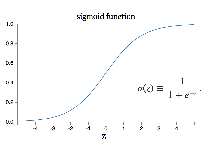
What if, on the other hand, a minor change in the weight results in a large change in the output? The sigmoid neuron model is capable of resolving this issue.
Applications of Feedforward Neural Network
These neural networks are utilized in a wide variety of applications. Several of them are denoted by the following area units:
- Physiological feedforward system: Here, feedforward management is exemplified by the usual preventative control of heartbeat prior to exercise by the central involuntary system.
- Gene regulation and feedforward: Throughout this, a theme predominates throughout the famous networks, and this motif has been demonstrated to be a feedforward system for detecting non-temporary atmospheric alteration.
- Automating and managing machines
- Parallel feedforward compensation with derivative: This is a relatively recent approach for converting the non-minimum component of an open-loop transfer system into the minimum part.
Conclusion
Deep learning is a field of software engineering that has accumulated a massive amount of study over the years. There are several neural network designs that have been developed for use with diverse data kinds. Convolutional neural systems, for example, have achieved best-in-class performance in the disciplines of image handling processes, while recurrent neural systems are commonly used in the fields of content and speech processing.
When applied to large datasets, neural networks require enormous amounts of computing power and equipment acceleration, which may be achieved through the design of a system of graphics processing units, or GPUs, arranged in a cluster. Those who are new to the use of GPUs can find free customized settings on the internet, which they can download and use for free. They are Kaggle Notebooks and Google Collabor Notebooks, which are the most widely used.
In order to build a feedforward neural network that works well, it is necessary to test the network design several times in order to get it right.
I’m glad you found it interesting. In order to contact me, you may do so using the following methods:
If you still have questions, feel free to send them to me by e-mail.
The media shown in this article is not owned by Analytics Vidhya and are used at the Author’s discretion.


