


Time flies by! I see Jenika (my daughter) running around in the entire house and my office now. She still slips and trips – but is now independent to explore the world and figure out new stuff on her own. I hope I would have been able to inspire similar confidence with use of Python for data analysis in the followers of this series.
For those, who have been following, here are a pair of shoes for you to start running!

By end of this tutorial, you will also have all the tools necessary to perform any data analysis by yourself using Python.
Recap – Getting the basics right
In the previous posts in this series, we had downloaded and setup a Python installation, got introduced to several useful libraries and data structures and finally started with an exploratory analysis in Python (using Pandas).
In this Pandas tutorial, we will continue our journey from where we left it in our last tutorial – we have a reasonable idea about the characteristics of the dataset we are working on. If you have not gone through the previous article in the series, kindly do so before proceeding further.
Data munging – recap of the need
While our exploration of the data, we found a few problems in the dataset, which need to be solved before the data is ready for a good model. This exercise is typically referred as “Data Munging”. Here are the problems, we are already aware of:
- About 31% (277 out of 891) of values in Age are missing. We expect age to play an important role and hence would want to estimate this in some manner.
- While looking at the distributions, we saw that Fare seemed to contain extreme values at either end – a few tickets were probably provided free or contained data entry error. On the other hand $512 sounds like a very high fare for booking a ticket
In addition to these problems with numerical fields, we should also look at the non-numerical fields i.e. Name, Ticket and Cabin to see, if they contain any useful information.
Check missing values in the dataset
Let us look at Cabin to start with. First glance at the variable leaves us with an impression that there are too many NaNs in the dataset. So, let us check the number of nulls / NaNs in the dataset
[stextbox id = "grey"] sum(df['Cabin'].isnull()) [/stextbox]
This Pandas command should tell us the number of missing values as isnull() returns 1, if the value is null. The output is 687 – which is a lot of missing values. So, we’ll need to drop this variable.
Next, let us look at variable Ticket. Ticket looks to have mix of numbers and text and doesn’t seem to contain any information, so will drop Ticket as well.
[stextbox id = "grey"] df = df.drop(['Ticket','Cabin'], axis=1) [/stextbox]
How to fill missing values in Age using Pandas fillna?
There are numerous ways to fill the missing values of Age – the simplest being replacement by mean, which can be done by following code:
[stextbox id = "grey"] meanAge = np.mean(df.Age)
df.Age = df.Age.fillna(meanAge)[/stextbox]
The other extreme could be to build a supervised learning model to predict age on the basis of other variables and then use age along with other variables to predict survival.
Since, the purpose of this tutorial is to bring out the steps in data munging, I’ll rather take an approach, which lies some where in between these 2 extremes. The key hypothesis is that the salutations in Name, Gender and Pclass combined can provide us with information required to fill in the missing values to a large extent.
Here are the steps required to work on this hypothesis:
Step 1: Extracting salutations from Name
Let us define a function, which extracts the salutation from a Name written in this format:
Family_Name, Salutation. First Name
[stextbox id = "grey"]
def name_extract(word):
 return word.split(',')[1].split('.')[0].strip()
[/stextbox]
This function takes a Name, splits it by a comma (,), then splits it by a dot(.) and removes the whitespaces. The output of calling function with ‘Jain, Mr. Kunal’ would be Mr and ‘Jain, Miss. Jenika’ would be Miss
Next, we apply this function to the entire column using apply() function and convert the outcome to a new Pandas DataFrame df2:
[stextbox id = "grey"]
df2 = pd.DataFrame({'Salutation':df['Name'].apply(name_extract)})
[/stextbox]
Once we have the Salutations, let us look at their distribution. We use the good old groupby after merging the DataFrame df2 with DataFrame df:
[stextbox id = "grey"]
df = pd.merge(df, df2, left_index = True, right_index = True) # merges on index
temp1 = df.groupby('Salutation').PassengerId.count()
print temp1
[/stextbox]
Following is the output:
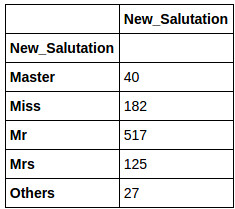
Salutation
Capt          1
Col           2
Don           1
Dr            7
Jonkheer      1
Lady          1
Major         2
Master       40
Miss        182
Mlle          2
Mme           1
Mr          517
Mrs         125
Ms            1
Rev           6
Sir           1
the Countess  1
dtype: int64
As you can see, there are 4 main Salutations – Mr, Mrs, Miss and Master – all other are less in number. Hence, we will combine all the remaining salutations under a single salutation – Others. In order to do so, we take the same approach, as we did to extract Salutation – define a function, apply it to a new column, store the outcome in a new Pandas DataFrame and then merge it with old DataFrame:
[stextbox id = "grey"]
def group_salutation(old_salutation):
if old_salutation == 'Mr':
return('Mr')
else:
if old_salutation == 'Mrs':
return('Mrs')
else:
if old_salutation == 'Master':
return('Master')
else:
if old_salutation == 'Miss':
return('Miss')
else:
return('Others')
df3 = pd.DataFrame({'New_Salutation':df['Salutation'].apply(group_salutation)})
df = pd.merge(df, df3, left_index = True, right_index = True)
temp1 = df3.groupby('New_Salutation').count()
temp1
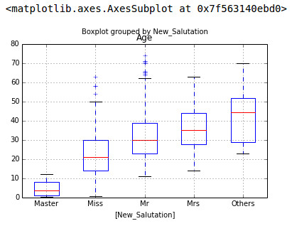
df.boxplot(column='Age', by = 'New_Salutation')
[/stextbox]
Following is the outcome for Distribution of New_Salutation and variation of Age across them:
Step 2: Creating a simple grid (Class x Gender) x Salutation
Similarly plotting the distribution of age by Sex & Class shows a sloping:
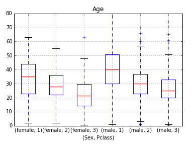
So, we create a Pivot table, which provides us median values for all the cells mentioned above. Next, we define a function, which returns the values of these cells and apply it to fill the missing values of age:
[stextbox id = "grey"]
table = df.pivot_table(values='Age', index=['New_Salutation'], columns=['Pclass', 'Sex'], aggfunc=np.median)
# Define function to return value of this pivot_table
def fage(x):
    return table[x['Pclass']][x['Sex']][x['New_Salutation']]
# Replace missing values
df['Age'].fillna(df[df['Age'].isnull()].apply(fage, axis=1), inplace=True)
[/stextbox]
This should provide you a good way to impute missing values of Age.
How to treat for Outliers in distribution of Fare?
Next, let us look at distribution of Fare by Pclass:
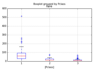
As expected the means of Fare line up neatly by Pclass. However, there are a few extreme values. One particular data point which grabs attention, the fare of 512 for Class 1 – this looks like a likely error. Again there are multiple ways to impute this data – replace by mean / median of Class 1 or you can also replace the value by the second highest value, which is closer to other data points.
You can choose you pick and replace the values. The commands are similar to the ones mentioned above.
End Notes:
Now our dataset is ready for building predictive models. In the next tutorial in this series, we will try out various predictive modeling techniques to predict survival of Titanic passengers and compare them to find out the best technique.
A quick recap, by now – you would be comfortable performing exploratory analysis and Data Munging in Pandas. Some of the steps in this tutorial can feel overdone for this problem – the idea was to provide a tutorial, which can help you even on bigger problems. If you have any other tricks, which you use for data cleaning and munging, please feel free to share them through comments below.
If you want to stay updated on latest analytics jobs, follow our job postings on twitter or like our Careers in Analytics page on Facebook
Kunal is a post graduate from IIT Bombay in Aerospace Engineering. He has spent more than 10 years in field of Data Science. His work experience ranges from mature markets like UK to a developing market like India. During this period he has lead teams of various sizes and has worked on various tools like SAS, SPSS, Qlikview, R, Python and Matlab.