This article was published as a part of the Data Science Blogathon
We are using Jupyter notebook to run our code. We suggest following this tutorial on Google Colaboratory. You can check out this link for more info about its usage.
To follow through this tutorial prior knowledge of PyTorch and python programming is assumed. No prerequisite knowledge of machine learning is required. You can check our previous blog on PyTorch to get acquainted with it.
Introduction to Linear Regression
Back Propagation is a powerful technique used in deep learning to update the weights and bias, thus enabling the model to learn. To better illustrate backpropagation, let’s look at the implementation of the Linear Regression model in PyTorch
Linear Regression is one of the basic algorithms in machine learning. Linear Regression establishes a linear relationship between input features (X) and output labels (y).
In linear regression, each output label is expressed as a linear function of input features which uses weights and biases. These weights and biases are the model parameters that are initialized randomly but then get updated through each cycle of training/learning through the dataset. Training the model and updating the parameters after going through a single iteration of training data is known as one epoch. So now we should train the model for several epochs so that weights and biases can learn the linear relationship between the input features and output labels.
So for this tutorial let’s create a model on hypothetical data consisting of crop yields of Mangoes and Oranges given the average Temperature, annual Rainfall and Humidity of a particular place. Training data is as follows:
| Region | Temperature (F) | Rainfall (mm) | Humidity (%) | Mangoes (ton) | Oranges (ton) |
| A | 73 | 67 | 43 | 56 | 70 |
| B | 91 | 88 | 64 | 81 | 101 |
| C | 87 | 134 | 58 | 119 | 133 |
| D | 102 | 43 | 37 | 22 | 37 |
| E | 69 | 96 | 70 | 103 | 119 |
| F | 74 | 66 | 43 | 57 | 69 |
| G | 91 | 87 | 65 | 80 | 102 |
| H | 88 | 134 | 59 | 118 | 132 |
| I | 101 | 44 | 37 | 21 | 38 |
| J | 68 | 96 | 71 | 104 | 118 |
| K | 73 | 66 | 44 | 57 | 69 |
| L | 92 | 87 | 64 | 82 | 100 |
| M | 87 | 135 | 57 | 118 | 134 |
| N | 103 | 43 | 36 | 20 | 38 |
| O | 68 | 97 | 70 | 102 | 120 |
In linear regression, each target label is expressed as a weighted sum of input variables along with a bias i.e
Mangoes = w11 * temp + w12 * rainfall + w13 * humidity + b1
Oranges = w21 * temp + w22 * rainfall + w23 * humidity + b2
Initially, the weights and biases are initialised randomly, and then they are updated accordingly during the training process so that those weights and biases predict the amount of Mangoes and oranges produced in any region given the temperature, rainfall, and humidity up to some levels of accuracy.
This in nutshell is Machine learning.
So now let’s get started with implementation using Pytorch…
Imports
Import the required libraries
import torch
import numpy as np
Load the Data
The training data given in the above table can be represented as matrices using NumPy. So let’s define inputs and targets separately,
inputs = np.array([[73, 67, 43],
                   [91, 88, 64],
                   [87, 134, 58],
                   [102, 43, 37],
                   [69, 96, 70],
                   [74, 66, 43],
                   [91, 87, 65],
                   [88, 134, 59],
                   [101, 44, 37],
                   [68, 96, 71],
                   [73, 66, 44],
                   [92, 87, 64],
                   [87, 135, 57],
                   [103, 43, 36],
                   [68, 97, 70]],
                  dtype='float32')
targets = np.array([[56, 70],
                    [81, 101],
                    [119, 133],
                    [22, 37],
                    [103, 119],
                    [57, 69],
                    [80, 102],
                    [118, 132],
                    [21, 38],
                    [104, 118],
                    [57, 69],
                    [82, 100],
                    [118, 134],
                    [20, 38],
                    [102, 120]],
                   dtype='float32')
Both the input and target matrices are loaded as NumPy arrays. This is should be converted to torch tensors using the torch.from_numpy() method,
inputs = torch.from_numpy(inputs)
targets = torch.from_numpy(targets)
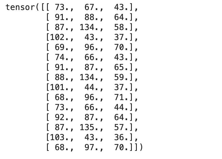
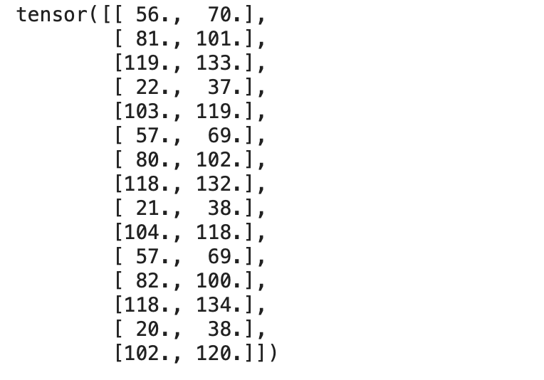
We can check both the tensors,
print(inputs)
Output:
print(targets)
Output:
Now let’s create a TensorDataset, which wraps inputs and targets tensors into a single dataset. Let’s import TensorDataset method from torch.utils.data. We can access rows from the dataset as tuples.
from torch.utils.data import TensorDataset
dataset = TensorDataset(inputs, targets)
We can access the rows of inputs and corresponding targets from a defined dataset using indexing as in Python.
dataset[:3]

Now let’s convert the dataset into a dataloader that can split the data into batches of predefined batch size during training.
Using Pytorch’s DataLoader class we can convert the dataset into batches of predefined batch size and create batches by picking samples from the dataset randomly.
from torch.utils.data import DataLoader

batch_size = 3
train_loader = DataLoader(dataset, batch_size=batch_size, shuffle=True)
We can access the data from DataLoader as a tuple pair containing input and corresponding targets using a for loop which enables us to load batches directly into a training loop.
# A Batch Sample
for inp,target in train_loader:
    print(inp)
    print(target)
    break
Output:

Now as our data is ready for training let’s define the Linear Regression Algorithm.
Linear Regression – From Scratch
In statistical modeling, regression analysis is a set of statistical processes for estimating the relationships between a dependent variable and one or more independent variables. -Wikipedia
Let’s implement a linear regression model from scratch. We should find the optimal weights and biases which is specified in the above equations so that it defines the ideal linear relationship between inputs and outputs.
So we define a set of weights as in the above equation to establish a linear relationship with input features and targets. Here we also set the requires_grad property of hyperparameters (i.e. weights and biases) to True.
w = torch.randn(2, 3, requires_grad=True)
b = torch.randn(2, requires_grad=True)
print(w)
print(b)
Output:

torch.randn generates tensors randomly from a uniform distribution with mean 0 and standard deviation 1.
The equation of Linear Regression is y = w * X + b, where
- y is the output or dependent variable
- X is the input or independent variable
- w & b are the weights and biases respectively
Therefore now let’s define our Linear Regression model,
def model(X):
    return X @ w.t() + b
The model is just a mathematical equation establishing a linear relationship between weights and outputs.
Matrix multiplication is performed ( @ represents matrix multiplication) with the input batch and the transpose of the weights.
Now let’s predict the model’s output for a batch of data,
for x,y in train_loader:
    preds = model(x)
    print("Prediction is :n",preds)
    print("nActual targets is :n",y)
    break
Output:

We can see above that our model is predicting values that differ from actual targets by a huge margin since our model is initialised with random weights and biases. Obviously, we can’t expect our randomly initialised model to perform well.
Loss Function
The loss function is the measure of how well the model is performing. Loss function plays an important role in updating the hyperparameters so that the resulting loss will be less.
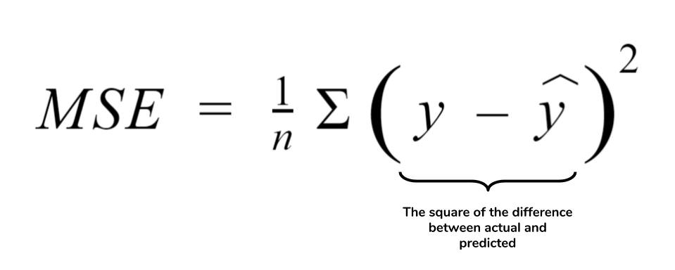
One of the most widely used loss functions for Regression is Mean Squared Error or L2 loss. MSE defines the mean of the square of the difference between actual and the predicted values. It is given as follows:
def mse_loss(predictions, targets):
    difference = predictions - targets
    return torch.sum(difference * difference)/ difference.numel()
.numel() method returns the number of elements in the tensor.
Now let’s make a prediction and compute the loss of our untrained model,
for x,y in train_loader:
    preds = model(x)
    print("Prediction is :n",preds)
    print("nActual targets is :n",y)
    print("nLoss is: ",mse_loss(preds, y))
    break
Output:
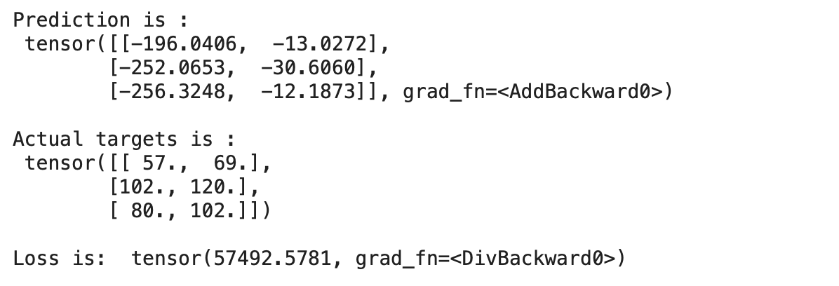
We can see that our prediction is varying from the actual targets with a huge margin which indicates that the loss of the model is huge.
Hence we should update the weights and biases so that the loss reduces. This can be done by using an optimization algorithm called Gradient Descent.
Gradient Descent
Gradient descent is a first-order iterative optimization algorithm for finding a local minimum of a differentiable function. The idea is to take repeated steps in the opposite direction of the gradient (or approximate gradient) of the function at the current point, because this is the direction of steepest descent. – Wikipedia
Gradient descent is an optimization algorithm that calculates the derivative/gradient of the loss function to update the weights and correspondingly reduce the loss or find the minima of the loss function.
Steps to implement Gradient Descent in PyTorch,
- First, calculate the loss function
- Find the Gradient of the loss with respect to independent variables
- Update the weights and bais
- Repeat the above step
Now let’s get into coding and implement Gradient Descent for 50 epochs,
epochs = 50
for i in range(epochs):
    # Iterate through training dataloader
    for x,y in train_loader:
        # Generate Prediction
        preds = model(x)
        # Get the loss and perform backpropagation
        loss = mse_loss(preds, y)
        loss.backward()
        # Let's update the weights
        with torch.no_grad():
            w -= w.grad *1e-6
            b -= b.grad * 1e-6
            # Set the gradients to zero
            w.grad.zero_()
            b.grad.zero_()
     print(f"Epoch {i}/{epochs}: Loss: {loss}")
Output:
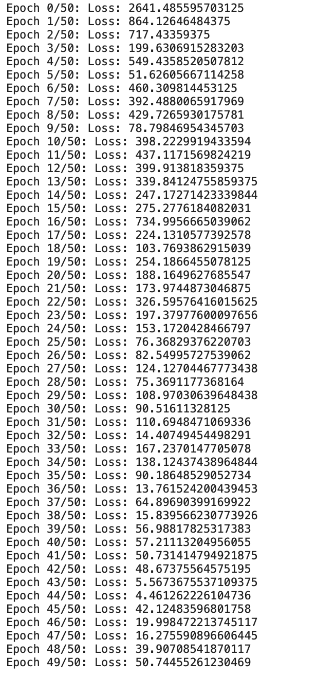
Now we can see that our custom-built linear regression model from scratch is training for the given data.
We can see that the loss has been gradually decreasing. Now let’s check the output once,
for x,y in train_loader:
    preds = model(x)
    print("Prediction is :n",preds)
    print("nActual targets is :n",y)
    break
Output:

We can see that the prediction is almost close to the actual targets. We are able to predict this by training/updating weights and biases of our Linear Regression Model for 50 epochs.
Conclusion
This process of updating the weights/parameters using gradient descent after every iteration of the dataset through our model based on loss defines the basis for Deep Learning, which can address the plethora of tasks including vision, images, text etc
About the Author:
I’m Narasimha Karthik, Deep Learning Practioner.
Currently working with Computer Vision and NLP. Experience in working with PyTorch, Fastai, Tensorflow and Keras frameworks. You can contact me through LinkedIn and Twitter for any projects or discussions.
The link for this notebook can be found here.
Thank you


