Introduction
While dealing with Linear Regression we can have multiple lines for different values of slopes and intercepts. But the main question that arises is which of those lines actually represents the right relationship between the X and Y and in order to find that we can use the Mean Squared Error or MSE as the parameter. For linear regression, this MSE is nothing but the Cost Function.
Mean Squared Error is the sum of the squared differences between the prediction and true value. And the output is a single number representing the cost. So the line with the minimum cost function or MSE represents the relationship between X and Y in the best possible manner. And once we have the slope and intercept of the line which gives the least error, we can use that line to predict Y.
So this article is all about calculating the errors/cost for various lines and then finding the cost function, which can be used for prediction.
Note: If you are more interested in learning concepts in an Audio-Visual format, We have this entire article explained in the video below. If not, you may continue reading.
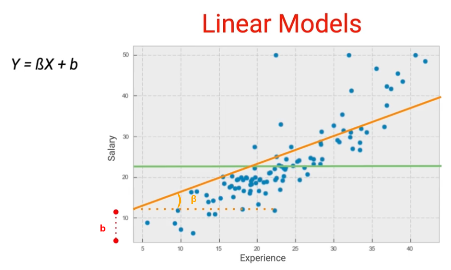
As we know that any line can be represented by two parameters- slope(β) and intercept(b).
And once we have a line we can always calculate the errors(also known as cost or loss) which this line would have from the underlying data point and the idea is to find the line which gives us the least error. This basically becomes an optimization problem. Let’s go through an exercise where you’ll see what is the error for various values of β and B and then the question is how do we find the most optimum values of these two parameters.
Let’s begin!
Importing Libraries
I’ll start by importing the necessary libraries which are matplotlib, pandas and scikit learn to calculate the error:
#import the libraries

import matplotlib.pyplot as plt
import pandas as pd
from sklearn.metrics import mean_squared_error as mse
Creating sample Data
And I have created a data set for Experience and Salary. For that, I’ve created a list and then just simply converted it to a Pandas Dataframe using pd.DataFrame():
Python Code:
You can see the first five rows of our dataset.
Plotting the data
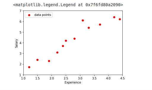
Let us now explore the dataset by exploring the relationship between salary and experience. Let’s plot this using Matplotlib:
# plotting the data

plt.scatter(data.experience, data.salary, color = 'red', label = 'data points')
plt.xlim(1,4.5)
plt.ylim(1,7)
plt.xlabel('Experience')
plt.ylabel('Salary')
plt.legend()
You can see a linear relationship between experience and salary. And this is what we expected. So let’s now start by plotting the lines by using various values of β and b.
Starting the Line using small values of parameters(beta and b)
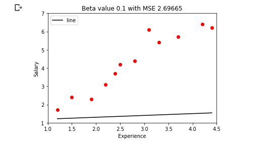
To start with let me take β = 0.1 and b = 1.1 and what I’m going to do is create a line with these two parameters and plot it over the scatter plot. Now, I take values and then apply this relationship to create each of these lines and then I plot this over the above-created scatter plot.
# making lines for different Values of Beta 0.1, 0.8, 1.5
beta = 0.1

# keeping intercept constant
b = 1.1

# to store predicted points
line1 = []

# generating predictions for every data point
for i in range(len(data)):
    line1.append(data.experience[i]*beta + b)

# Plotting the line
plt.scatter(data.experience, data.salary, color = 'red')
plt.plot(data.experience, line1, color = 'black', label = 'line')
plt.xlim(1,4.5)
plt.ylim(1,7)
plt.xlabel('Experience')
plt.ylabel('Salary')
plt.legend()

MSE = mse(data.salary, line1)

plt.title("Beta value "+str(beta)+" with MSE "+ str(MSE))

MSE = mse(data.salary, line1)
We have this line for beta = 0.1 and b = 1.1 and the MSE for this line is 2.69. Now as you can see the slope of the line is very less so I would want to actually try out a higher slope so instead of beta = 0.1 let me change this to beta = 1.5 :
This is the line for beta = 1.5 and b = 1.1 and the MSE for this line is 6.40. You can see a better slope but it is probably more than what we actually want. So the right value might be somewhere in between 0.1 and1.5, so let’s try beta = 0.8:
This is the line with beta = 0.8 and b = 1.1 and we can see that the mean squared error has come down to 0.336
We have tried 3 different lines with each of these having different MSE; the first one had 2.69, the second had 6.4 and the third one had 0.33. Now we can go on and try this for various values of beta. So now we can try this with various values of Beta and see what is the relationship between beta and mean squared error(MSE), for a fixed value intercept i.e b. So we’re not changing b.
Computing Cost Function over a range of values of Beta
So let’s create a function which I am calling as Error and what this function does is for a given value beta it is basically giving me what is the MSE for these data points. Here b is fixed and I am trying different values of Beta.
# function to calculate error

def Error(Beta, data):

# b is constant
    b = 1.1

    salary = []
    experience = data.experience

# Loop to calculate predict salary variables
    for i inrange(len(data.experience)):
        tmp = data.experience[i] * Beta + b
        salary.append(tmp)

MSE = mse(data.salary, salary)
return MSE
Now I am trying all values of Beta between 0 to 1.5 with an increment of 0.01 and I’ll then append everything to a list:
# Range of slopes from 0 to 1.5 with increment of 0.01

slope = [i/100 for i in range(0,150)]
Cost = []
for i in slope:
    cost = Error( Beta = i, data = data)
    Cost.append(cost)
Visualizing cost with respect to Beta
When this is done, just convert this into this is the Data Frame:
# Arranging in DataFrame

Cost_table = pd.DataFrame({
'Beta' : slope,
'Cost' : Cost
})

Cost_table.head()
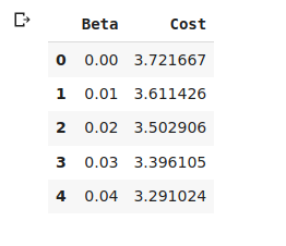
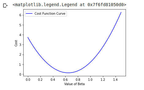
What this data frame is showing that for a value of Beta which is 0.00 the cost or MSE we’re getting is 3.72, similarly for beta = 0.04, we are getting cost = 3.29. Let’s quickly visualize this:
# plotting the cost values corresponding to every value of Beta

plt.plot(Cost_table.Beta, Cost_table.Cost, color = 'blue', label = 'Cost Function Curve')
plt.xlabel('Value of Beta')
plt.ylabel('Cost')
plt.legend()
This is the plot which we get. So as you can see the value of cost at 0 was around 3.72, so that is the starting value. After that the error goes down with the increasing value of Beta, reaches a minimum, and then it starts increasing.
Now the question is given that we know this relationship, what are the values of beta and b for which we can find out this particular location where my cost is minimum.
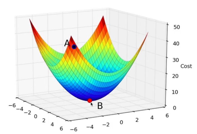
Now what happens when you have two parameters, I mean right now we assumed b to be 0.1 but actually what we want to do is change it with respect to b as well as beta and in this particular situation this is the curve which we get:
So again, this is just a 3D plot, so you have two dimensions but it will again have a minimum value and the idea would be to find the minimum value. But you cannot do this iteratively in the way we did so far. So what we need to find is a smarter way in which we can find this minimum value and that is where the Gradient Descent technique comes into play.
End Notes
In this article, you learned how to calculate the error for various lines and how to find the optimum line.
If you are looking to kick start your Data Science Journey and want every topic under one roof, your search stops here. Check out Analytics Vidhya’s Certified AI & ML BlackBelt Plus Program
This article concluded with the introduction of a new term Gradient Descent, which will be covered in upcoming articles. So, stay tuned!


