


This article was published as a part of the Data Science Blogathon.
In this article, we will learn RNN, LSTM, Bidirectional LSTM and GRU in detail with the implementation of movie sentiment classification.
Introduction
In NLP we have seen some NLP tasks using traditional neural networks, like text classification, sentiment analysis, and we did it with satisfactory results. but this wasn’t enough, we faced certain problems with traditional neural networks as given below.
1. The prediction was highly dependent on the specific words.
2. If you change any word with it synonyms result gets deviated.
3. If you write like, affection instead of love, the result gets deviated.
4. The prediction was not dependent on the sequence of words.
To fix this problem we came up with the idea of Word Embedding and a model which can store the sequence of the words and depending on the sequence it can generate results.
ie “I love playing Ball” and “I do not love playing Ball”
In both the sentence we see “love” hence our vanilla model can classify it as a positive sentiment but as you see its negative sentiment, here sequence of words matters a lot. So far we had no model which can consider the sequence of words in a sentence for the prediction.
RNN ( Recurrent Neural Networks)
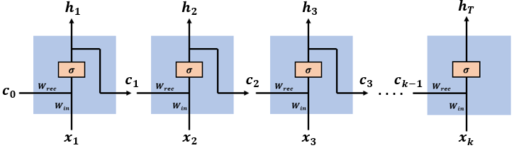
Source: OpenSource
To solve this problem RNN came into the picture. which solves this problem by using hidden layers. and hidden layers are the main features of RNN. hidden layers help RNN to remember the sequence of words (data) and use the sequence pattern for the prediction.
The idea of RNN has developed a lot. it has been used for speech recognition and various NLP tasks where the sequence of words matters. RNN takes input as time series (sequence of words ), we can say RNN acts like a memory that remembers the sequence.
Use cases of RNN
- Speech, text recognition & sentiment classification
- Music synthesis
- Image captioning
- Chatbots & NLP
- Machine Translation — Language translation
- Stock predictions
- Finding and blocking abusive words in a speech or text
Does RNN sound so powerful? No ! there is a big problem.
Problems with RNN :
Exploding and vanishing gradient problems during backpropagation.
Gradients are those values which to update neural networks weights. In other words, we can say that Gradient carries information.
Vanishing gradient is a big problem in deep neural networks. it vanishes or explodes quickly in earlier layers and this makes RNN unable to hold information of longer sequence. and thus RNN becomes short-term memory.
If we apply RNN for a paragraph RNN may leave out necessary information due to gradient problems and not be able to carry information from the initial time step to later time steps.
To solve this problem LSTM, GRU came into the picture.
How do LSTM, GRU solve this problem?
I highly encourage you to read Colah’s blog for in-depth knowledge of LSTM.
The reason for exploding gradient was the capturing of relevant and irrelevant information. a model which can decide what information from a paragraph and relevant and remember only relevant information and throw all the irrelevant information
This is achieved by using gates. the LSTM ( Long -short-term memory ) and GRU ( Gated Recurrent Unit ) have gates as an internal mechanism, which control what information to keep and what information to throw out. By doing this LSTM, GRU networks solve the exploding and vanishing gradient problem.
Almost each and every SOTA ( state of the art) model based on RNN follows LSTM or GRU networks for prediction.
LSTMs /GRUs are implemented in speech recognition, text generation, caption generation, etc.
LSTM networks
Every LSTM network basically contains three gates to control the flow of information and cells to hold information. The Cell States carries the information from initial to later time steps without getting vanished.
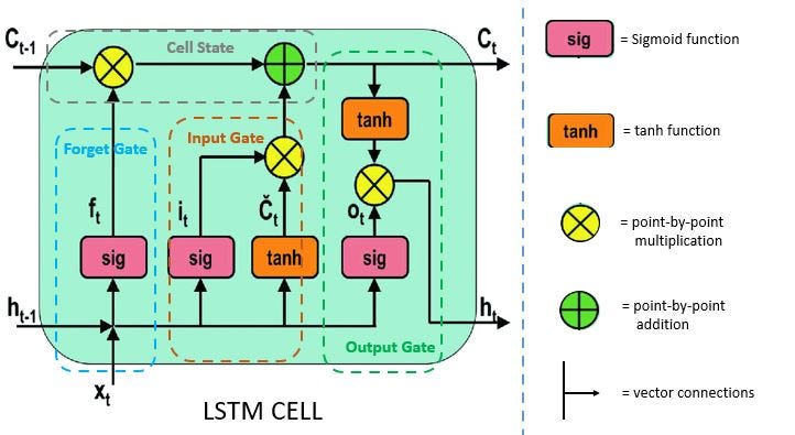
Gates
Gates make use of sigmoid activation or you can say tanh activation. values ranges in tanh activation are 0 -1.
- Forget Gate
- Input Gate
- Output Gate
Let’s see these gates in detail:
- Forget Gate:
This gate decides what information should be carried out forward or what information should be ignored.
Information from previous hidden states and the current state information passes through the sigmoid function. Values that come out from sigmoid are always between 0 and 1. if the value is closer to 1 means information should proceed forward and if value closer to 0 means information should be ignored.
2. Input Gate:
After deciding the relevant information, the information goes to the input gate, Input gate passes the relevant information, and this leads to updating the cell states. simply saving updating the weight.
Input gate adds the new relevant information to the existing information by updating cell states.
3. Output Gate:
After the information is passed through the input gate, now the output gate comes into play. Output gate generates the next hidden states. and cell states are carried over the next time step.
GRU
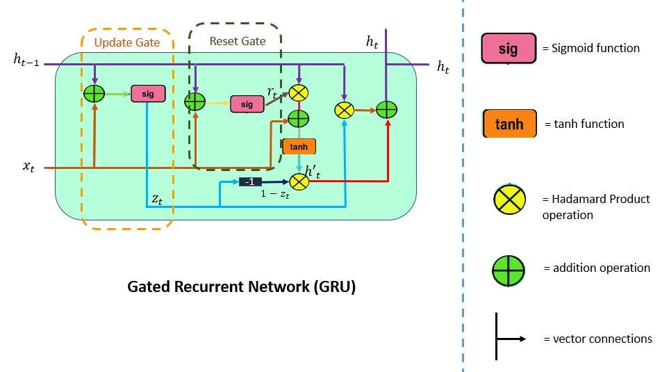
GRU ( Gated Recurrent Units ) are similar to the LSTM networks. GRU is a kind of newer version of RNN. However, there are some differences between GRU and LSTM.
- GRU doesn’t contain a cell state
- GRU uses its hidden states to transport information
- It Contains only 2 gates(Reset and Update Gate)
- GRU is faster than LSTM
- GRU has lesser tensor’s operation that makes it faster
1. Update Gate
Update Gate is a combination of Forget Gate and Input Gate. Forget gate decides what information to ignore and what information to add in memory.
2. Reset Gate
This Gate Resets the past information in order to get rid of gradient explosion. Reset Gate determines how much past information should be forgotten.
BI-LSTM Networks
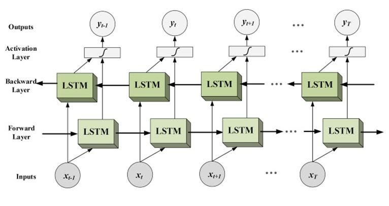
We have seen how LSTM works and we noticed that it works in uni-direction.
Bidirectional long-short term memory networks are advancements of unidirectional LSTM. Bi-LSTM tries to capture information from both sides left to right and right to left. The rest of the concept in Bi-LSTM is the same as LSTM.
This improves the accuracy of models.
Implementation
We are going to perform a movie review (text classification) using BI-LSTM on the IMDB dataset. The goal is to read the review and predict if the user liked it or not.
- Importing Libraries
import numpy as np
from keras.models import Sequential
from keras.preprocessing import sequence
from keras.layers import Dropout
from keras.layers import  Dense, Embedding, LSTM, Bidirectional
2. Importing the dataset
Loading IMDB standard dataset using the Keras dataset class.
from keras.datasets import imdb
(x_train, y_train),(x_test, y_test) = imdb.load_data(num_words=10000)
num_words = 10000 signifies that only 10000 unique words will be taken for our dataset.
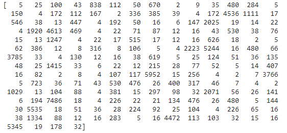
x_train, x_test: List of movie reviews text data. having an uneven length.
y_train, y_test: Lists of integer target labels (1 or 0).
3. Feature Extraction
Since we have text data in x_train and x_test of having an uneven length. Our goal is to convert this text data into a numerical form in order to feed it into the model.
Make the length of texts equal using padding.
We are defining max_len = 200. If a sentence is having a length greater than 200 it will be trimmed off otherwise it will be padded by 0.
max_len = 200
x_train = sequence.pad_sequences(x_train, maxlen=maxlen)
x_test = sequence.pad_sequences(x_test, maxlen=maxlen)
y_test = np.array(y_test)
y_train = np.array(y_train)
4. Designing the Bi-directional LSTM
The way we will be defining our bidirectional LSTM will be the same for LSTM as well.
You can either use Sequential or Functional API to create the model. here we are using Sequential API.
model = Sequential()
model.add(Embedding(n_unique_words, 128, input_length=maxlen))
model.add(Bidirectional(LSTM(64)))
model.add(Dropout(0.5))
model.add(Dense(1, activation='sigmoid'))
model.compile(loss='binary_crossentropy', optimizer='adam', metrics=['accuracy'])
input_length = maxlenSince we have already made all sentences in our dataset have an equal length of 200 using pad_sequence.- The Embedding layer takes
n_unique_wordsas the size of the vocabulary in our dataset which we already declared as 10000. - After the Embedding layer, we are adding Bi-directional LSTM units.
- Using sigmoid activation and then compiling the model
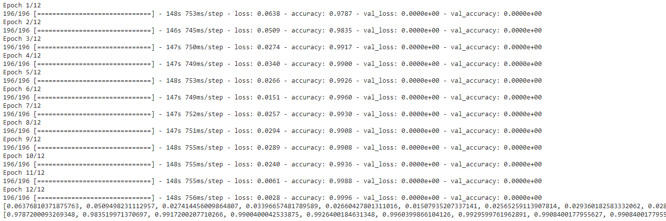
5. Training the model
We have prepared our dataset and model not calling the fit method to train our model.
history=model.fit(x_train, y_train,
           batch_size=batch_size,
           epochs=12,
           validation_data=[x_test, y_test])
print(history.history['loss'])
print(history.history['accuracy'])
6. Result
The plotting result can tell us how effective our training was. Let’s plot the training results.
from matplotlib import pyplot
pyplot.plot(history.history['loss'])
pyplot.plot(history.history['accuracy'])
pyplot.title('model loss vs accuracy')
pyplot.xlabel('epoch')
pyplot.legend(['loss', 'accuracy'], loc='upper right')
pyplot.show()
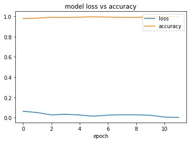
As you can see the accuracy line is nearly touching the one and loss is minimum very close to zero. However, you can go ahead and draw some predictions using the model.
Conclusion
In this article, we learned about RNN, LSTM, GRU, BI-LSTM and their various components, how they work and what makes them keep an upper hand for NLP tasks. We saw the implementation of Bi-LSTM using the IMDB dataset which was ideal for the implementation didn’t need any preprocessing since it comes with the Keras dataset class. If you have something to ask me write to me on Linkedin.
Read more about RNN here.
References:
- https://towardsdatascience.com/illustrated-guide-to-lstms-and-gru-s-a-step-by-step-explanation-44e9eb85bf21
- https://analyticsindiamag.com/complete-guide-to-bidirectional-lstm-with-python-codes/
Image Sources:
- https://analyticsindiamag.com/complete-guide-to-bidirectional-lstm-with-python-codes/
- https://towardsdatascience.com/illustrated-guide-to-lstms-and-gru-s-a-step-by-step-explanation-44e9eb85bf21