This article was published as a part of the Data Science Blogathon.
Table of Contents
1. Introduction
2. Decision Tree
3. Terminologies
4. CART Algorithm
5. Calculating Information Gain
6. Implementation
7. Conclusion
Introduction
This article discusses the Decision Tree machine learning algorithm in the field of artificial intelligence. In this article, I will try to cover everything related to it. First of all, let’s see what is classification.
Classification: The process of dividing the data points into the data set into different groups or different categories by adding a label to it is called Classification.
To which group the data point is added will be decided based on some condition. In other words, it is the technique of categorizing the observations into different categories.
Example: We all use Gmail. In that, all the mails are categorized as either spam or ham. It is done using the classification technique.
Classification is used for protection like checking whether the transaction is genuine or not. If your debit card is from India and if you use that card in foreign countries then it will send you a notification alert about it. This is done because it identified the transaction as not genuine.
Some of the Classification algorithms are
1. Decision Tree
2. Random Forest
3. Naive Bayes
4. KNN
5. Logistic Regression
6. SVM
In which Decision Tree Algorithm is the most commonly used algorithm.
Decision Tree
Decision Tree: A Decision Tree is a supervised learning algorithm. It is a graphical representation of all the possible solutions. All the decisions were made based on some conditions.
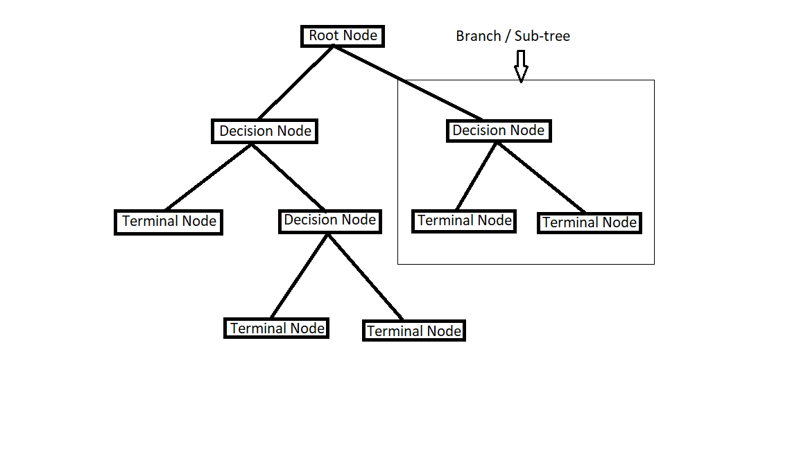
Do you know why this algorithm is known as a Decision Tree??? Because it starts from the root node and branches off to the number of solutions just like a tree. The tree also starts from the root and it starts growing its branches when it grows bigger and bigger.
To understand more, Take this example which is represented in a tree model below.
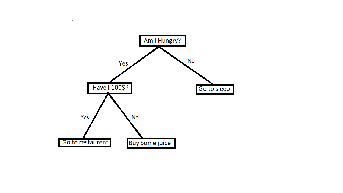
Here the root node is a question asking whether you are hungry or not. If you are not hungry then go back to sleep. If you are hungry then check whether you have 100 dollars or not. If you have sufficient money then go to the restaurant. If you don’t have enough money then go and just buy some juice.
In this way, the Decision Tree divides into different groups based on some conditions.
Let us take a dataset to understand more.
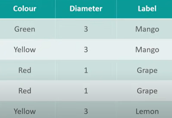
In this dataset, we can see fruits were labelled into either Mango, Grape, or Lemon based on colour and Diameter.
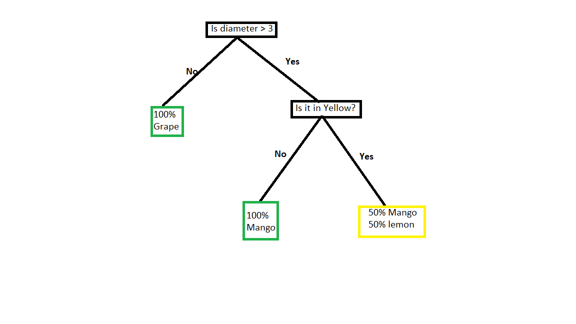
Here we take the root node as diameter. If the diameter is greater than 3 then we have colour as either Green or yellow. and so if the diameter is less than 3 then for sure it is grape which is red.
Now we have to check the colour. If it is not yellow then for sure it is mango. But if it is in yellow then we have two options. it can be either mango or lemon. So there is a chance for 50% mango and 50% Lemon.
But which question comes as the root node and which question comes next? Here we need to see which attribute will unmix the label at that particular point. We can find the amount of uncertainty at a single node with something known as Gini impurity and also we can find how much a question reduces that uncertainty with something known as Information Gain.
We use these to decide which question is asked and at which point
Terminologies
Root node: The root node is the base node of the tree where the entire tree starts from it.
Terminal Node/Leaf Node: This is the final node where no further segregation is possible.
Branch/Sub-tree: A branch is formed by splitting a node.
Pruning: Pruning is the opposite of splitting. Pruning is the process of removing nodes to decrease the size of the decision tree.
Parent Node/Child Node: Always root node is the parent node and all the other nodes which are derived from the parent node are known as child nodes.
CART Algorithm
CART(Classification and Regression Tree) algorithm is a predictive model which shows how an outcome of a variable is predicted based on other values.
Let’s have a look at this data.
Here there are attributes like Outlook, temperature, humidity, wind, and a label Play. All these attributes decide whether to play or not.
So among all of them which one should we pick first? The attribute which classifies the training data best will be picked first.
To decide that we need to learn some terms.
Gini Index: Gini Index is the measure of impurity or the purity that is used in building a decision tree in the CART Algorithm.
Information Gain: Information gain is the measure of how much information a feature gives about the class. It is the decrease in entropy after splitting the dataset based on the attribute.
Constructing a decision tree is all about finding the attribute that has the highest information gain.
Reduction in Variance: In general Variance is how much your data is varying. So here also attribute with a lower variance will be split first.
Chi-square: It is an algorithm to find the statistical significance of the differences between sub-nodes and parent nodes.
The first step to do before solving the problem for the decision tree is entropy which is used to find information gain. As we know splitting will be done based on information gain. Attribute with highest information gain is selected first.
Entropy: Entropy is the measure of uncertainty. It is a metric that measures the impurity of something.
Let’s understand what is impurity first.
Imagine a basket full of cherries and a bowl that contains labels with cherry written on it. Now if you take 1 fruit from the basket and 1 label from a bowl. So the probability of matching cherry with cherry is 1 and there is no impurity here.
Now imagine another situation with different fruits in a basket and different fruits names labels in the bowl. Now if you pick up 1 random fruit from the basket and 1 random label from the bowl, the probability of matching cherry with cherry is certainly not 1. It is less than 1. Here there is impurity.
Entropy=-ΣP(x)logP(x)
Entropy(s)=-P(yes)logP(yes)-P(no)logP(no)
where,
s = total sample space
P(yes) = Probability of yes
P(no) = Probability of no
If number of yes = number of no,T hen
P(s)=0.5 and Entropy(s) = 1
If it contains either all yes or all no, Then
P(s) = 1 or 0 and Entropy(s) = 0
let’s see first case, where number of yes = number of no
Entropy(s)=-P(yes)logP(yes)
E(s)=0.5 log20.5 – 0.5 log20.5
E(s)=0.5(log20.5 – log20.5)
E(s)=1
let’s see second case where it contains either all yes or all no
Entropy(s)=-P(yes)logP(yes)
E(s)=1log1
E(s)=0
Similarly with no.
Entropy(s)=-P(no)logP(no)
E(s)=1log1
E(s)=0
Calculating Information Gain
Information gain = Entropy(s) –[ (average weight) * Entropy(each feature)]
Let’s calculate the entropy for this dataset. Here total we have 14 data points in which 9 are yes and 5 are no.
Entropy(s)=-P(yes)logP(yes)-P(no)logP(no)
E(s)=-(9/14)log(9/14) – (5/14)log(5/14)
E(s)=0.41+0.53
E(s)=0.94
So entropy for this dataset is 0.94.
Now out of outlook, Temperature, Humidity, Windy which node is selected as a root node?
Let’s see one by one.
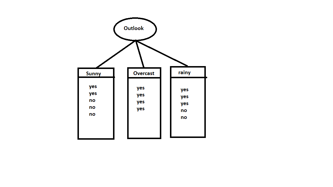
coming to outlook,
Here for sunny, we have 3 yes and 2 no. For Overcast, we have all yes. And for rainy we have 3 yes and 2 no.
E(outlook=sunny)=-2/5log2/5 – 3/5log3/5 = 0.971
E(outlook=Overcast)= -1log1 =0
E(outlook=rainy)=- 3/5log3/5 -2/5log2/5 =0.971
Information from outlook,
I(outlook)=5/14 * 0.971 + 4/14 * 0 + 5/14 * 0.971 = 0.693
Information gain from Outlook,
IG(Outlook)=E(s) -I(outlook)
=0.94 – 0.693
=0.247
So Information gain for outlook is 0.247.
Now lets consider windy as root node and calculate the information gain.
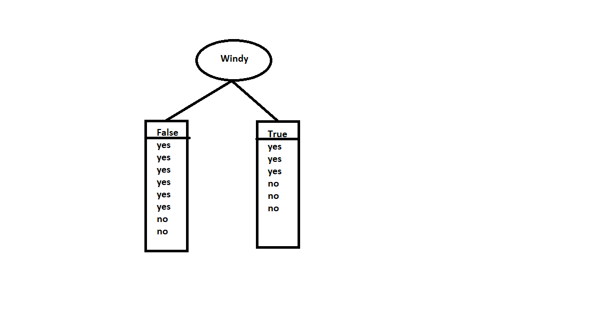
In the case of False, we have 6 yes and 2 no whereas in the case of True we have 3 yes and 3 no.
E(windy=True)=1
E(windy=False)=-6/8log6/8 -2/8log2/8 = 0.811
I(windy)=8/14 * 0.811 + 6/14 * 1 =0.892
IG(windy) = 0.94 – 0.892 = 0.048
So information gain for windy is 0.048.
Similarly, Calculate for others too.
Then finally you will get,
Information gain(Outlook) = 0.247
Information Gain(Temperature) = 0.029
Information Gain(Humidity) = 0.152
Information Gain(Windy) = 0.048
Attribute with highest information gain is selected. So here we can see information gain for outlook is more than remaining. So Outlook is selected as a root node.
We can observe that if the outlook is overcast then the final output will be yes. But if it is between sunny or rain, then again we have to calculate entropy for the remaining attributes and calculate the information gain to decide the next node. When all these calculations are done the final tree will look like this.
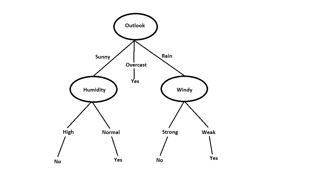
If Outlook is overcast then you can play without checking any other condition. If the outlook is sunny, then check for Humidity. If humidity is high, then don’t play. If humidity is normal then you can play. If the outlook is Rainy, then check for Windy conditions. If windy is strong then don’t play. If Windy is weak, then you can play.
Implementation
Now let’s see the code for it.
Source: Author
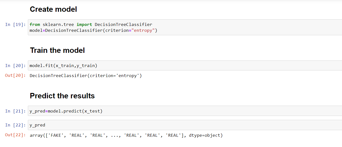
First, create a model by importing DecisionTreeClassifier from sklearn. Take entropy as a criterion for it. Then using training datasets, train the model. predict method predicts the outcome. You can see in the picture how it classifies between REAL and FAKE.
This is how the Decision Tree algorithm works.
Conclusion
In this article, we had discussed everything related to the decision tree algorithm. It is a classification algorithm used for supervised learning. And also it is easy to read and implement. We have seen some terminologies used in the decision tree algorithm like Gini index, Information gain, Chi-square. Further, we have seen how to build the decision tree using Information gain. And we have implemented the code in the Jupiter notebook using the scikit learn library.
Hope you guys found it useful.
Read more articles on the decision trees here.
Connect with me on Linkedin:
https://www.linkedin.com/in/amrutha-k-6335231a6vl/
The media shown in this article is not owned by Analytics Vidhya and are used at the Author’s discretion.


