This article was published as a part of the Data Science Blogathon.
Introduction to Classification Algorithms
In this article, we shall analyze loan risk using 2 different supervised learning classification algorithms. These algorithms are decision trees and random forests. At the outset, the basic features and the concepts involved would be discussed followed by a real-life problem scenario.
Classification with Decision Tree
A classifier in the form of a tree structure with 4 types of nodes viz. roots node, decision node, leaf node, and terminal node.
1. Root node – This node initiates the decision tree and represents the entire population that is being analyzed.
2. Decision node – This node specifies a choice or test of some attribute with each branch representing each outcome.
3. Leaf node – This node is an indicator of the classification of an example.
4. Terminal node – As the terminology suggests, it is the last node where the dataset cannot be classified anymore.
A representation of the above terminologies can be viewed in the image below
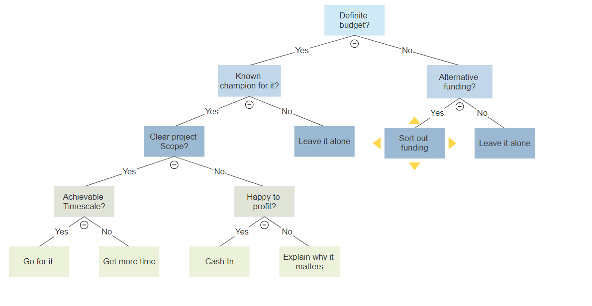
Constituents of a decision tree
The 3 most important ingredients to form a decision tree are
1) Entropy – is the measure of impurity of collection of examples and is dependent upon the distribution of the random variable. The value of entropy ranges between 0 and 1 where 0 indicates the certainty of the outcome and 1 indicates all possible outcomes are equally probable.
Entropy is mathematically represented as
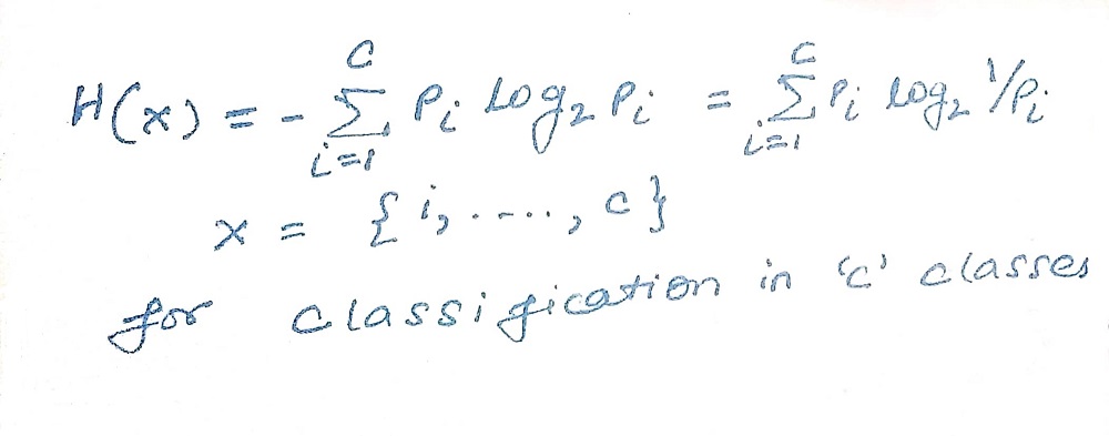
2) Information gain – is the anticipated reduction in entropy. Information gain is directly proportional to the attribute in classifying training data. Attribute having maximum information gain is selected as the splitting attribute.
Information gain is mathematically represented as
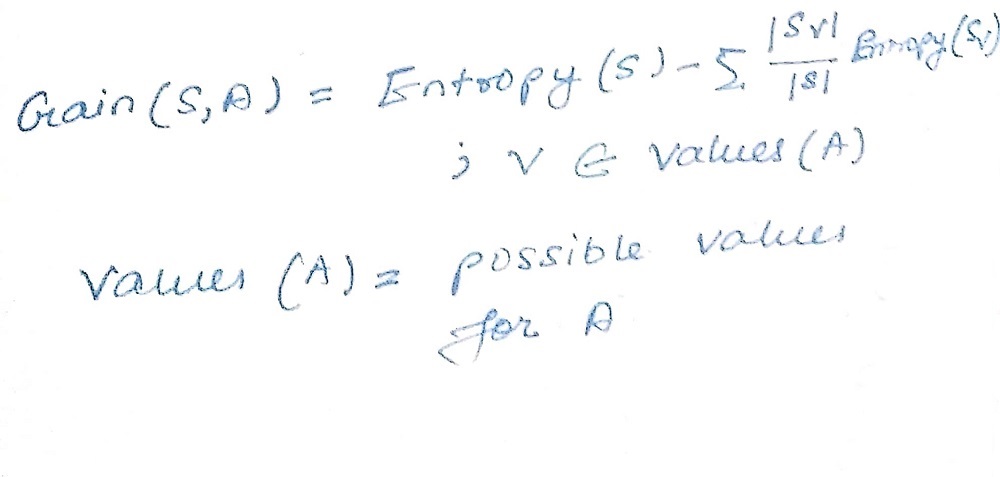
3) Gini index – is the measure of impurity and is based on Gini impurity. Mathematically, Gini impurity and gini index are represented as follows
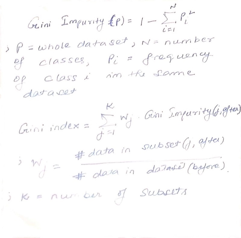
As can be seen in the formula above, the gini index is the weighted sum of the gini impurity of the subsets post-splitting and Gini impurity is 1 minus the sum of square of the class probabilities in a dataset.
Explanation of the underlying concepts of the constituents
1) Entropy – Let us consider a 1*1 matrix where a set of persons play badminton and a set of persons doesn’t
| Yes | No |
| 9 | 5 |
Now, Entropy(Play badminton) = Entropy(5,9) = Entropy(5/5+9,9/5+9) = Entropy(0.36,0.64)
Applying the formula of entropy, Entropy(Play badminton) = -(0.36 log20.36)-(0.64log20.64)
=0.4096+0.5292 = 0.9388 = 0.94
2) Information gain – Let us take the example of the badminton match being played or not depending upon certain conditions
| Play | badminton | Total | ||
| Yes | No | |||
| Outlook | Sunny | 3 | 2 | 5 |
| Overcast | 4 | 0 | 4 | |
| Rainy | 2 | 3 | 5 | |
| Total | 14 |
Entropy(Play badminton, Outlook) = P(Sunny)*E(3,2)+P(Overcast)*E(4,0)+P(Rainy)*E(2,3)
=(5/14)*0.971+(4/14)*0+(5/14)*0.971=0.693
Applying the formula of Information gain, G(Play badminton, Outlook) = 0.940-0.693
=0.247
| Play |
badminton | Total | ||
| Yes | No | |||
| Humidity | High | 3 | 4 | 7 |
| Low | 6 | 1 | 7 | |
| Total | 14 |
| Play | badminton | Total | ||
| Wind | Yes | No | ||
| False | 6 | 2 | 8 | |
| True | 3 | 3 | 6 | |
| Total | 14 |
| Play |
badminton | Total | ||
| Yes | No | |||
| Temperature | Hot | 2 | 2 | 4 |
| Mild | 4 | 2 | 6 | |
| Cool | 3 | 1 | 4 | |
| Total | 14 |
Calculation following similar procedure yields the following result
G(Play badminton, Humidity) = 0.151, G(Play badminton, Wind) = 0.084, G(Play badminton, Temp) = 0.029.
So, G(Play badminton, Outlook) will be chosen.
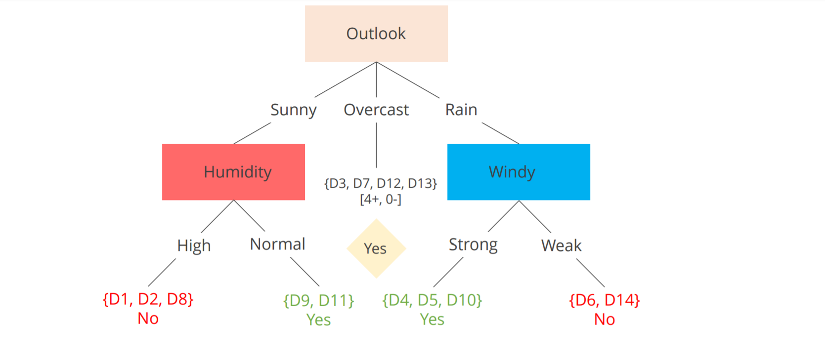
Then attributes within the outlook will be split further taking into consideration the gains and then finally at leaf nodes with a strong decision will be arrived upon as depicted below
3) Gini index – In a dataset having 2 classes, the range of the Gini index lies between 0 and 0.5. Here, 0 refers to a pure dataset and a value of 0.5 indicates 2 classes are distributed equally. Thus, the next split is dependent upon the feature with the lowest Gini index.
Challenges
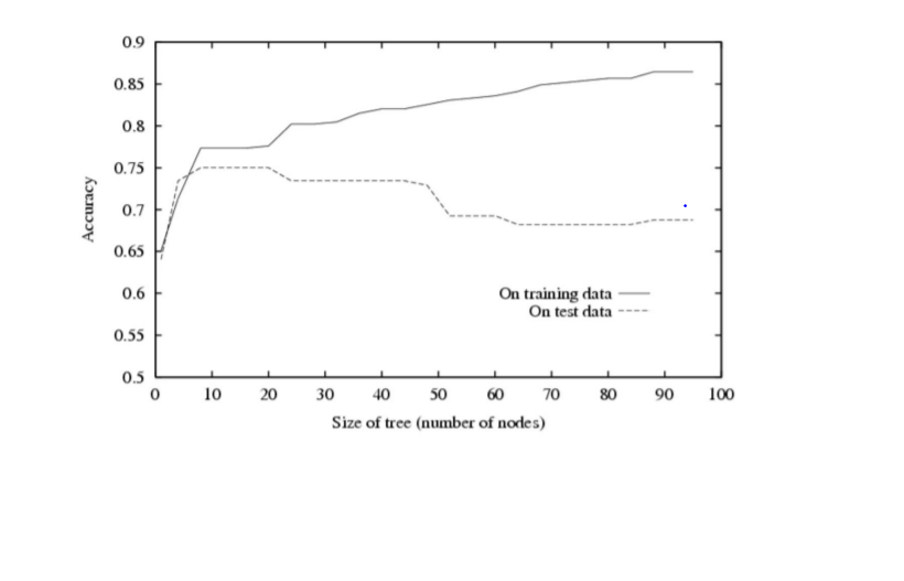
1) Size and overfitting – A decision tree that is too deep can make the model too detailed whereas a shallow decision tree can make a model very simple. Overfitting reduces training set error at the cost of an enlarged test set error.
Solution
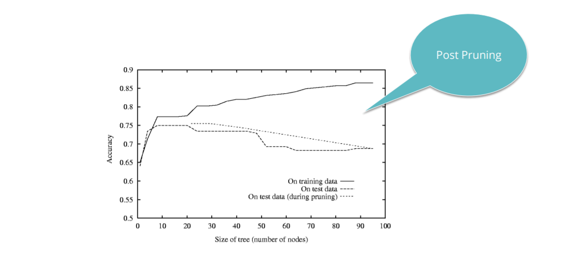
1) Pruning – is applied to a decision tree post-training phase. It allows the tree to grow as much as allowed without any restrictions. In the end, the branches are cut that are not populated sufficiently as these probably concentrate on special data points. So, removing them enables generalization on new unseen data.
2) Early stopping – A stopping criterion is used in this where the most common is the minimum number of samples per node.
Random Forest
The decision tree has evolved to give rise to a more robust performance-driven algorithm known as random forest. The concept behind the random forest algorithm is that many decision trees predict more accurately compared to an individual decision tree. The basis is multiple decision trees that are all trained differently to arrive at a final decision.
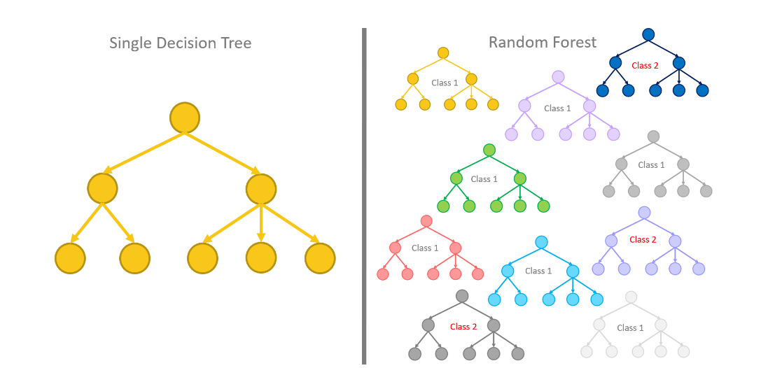 Image Source: https://www.knime.com/
1) Bagging – is a technique to reduce the variance of an estimated function of prediction. A vote is cast for each predicted class.
2)Bootstrapping – is a technique where datasets are being drawn randomly with replacement from the training data. All the samples are having a size similar to that of the original training set.Performance measures
1) Confusion matrix – It is a table used to comprehend the performance of a classification model.
| Predicted: Yes |
|
Total | |||
| Actual: Yes | a (T.P) | b (F.N) | a+b (Actual yes) | ||
| Actual: No | c (F.P) | d (T.N) | c+d (Actual No) | ||
| Total | a+c (Predicted yes) | b+d (Predicted No) | a+b+c+d |
2)Accuracy = a+d/a+b+c+d = T.P+T.N/Total
3)Precision = a/a+c = T.P/Predicted yes
4)Recall = a/a+b = T.P/Actual yes
Real-life case
There is an NBFC (Non-banking Financial Company) that connects borrowers and investors. As an investor, we want to invest in people who showed a profile of having a high probability of paying you back by creating a machine learning model that will help predict whether a borrower will pay the loan or not. The dataset is “loan_borowwer_data.csv”
We shall begin by importing the necessary libraries viz. pandas, and matplotlib.
import pandas as pd
import matplotlib.pyplot as plt
The, we would load the dataset
data=pd.read_csv('loan_borowwer_data.csv')
data.head()

We would check for the sum of missing values
data.isnull().sum()
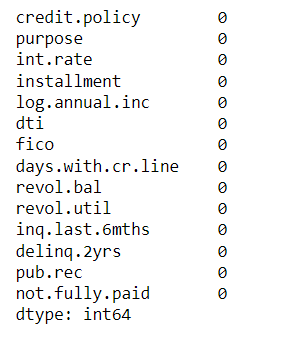
So, the dataset is not having missing values.
Now, we will use describe() function to calculate statistical data like percentile, mean, and std.
data.describe().T
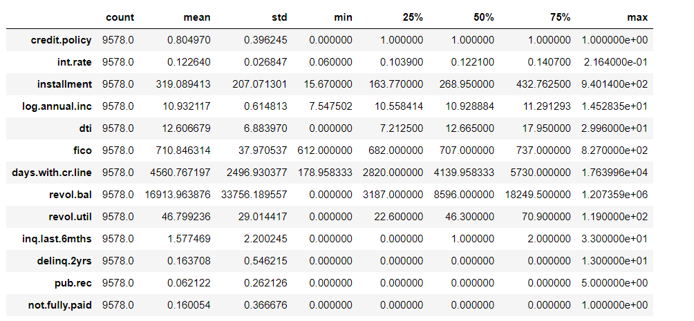
From the output, we know the mean, std, median, min, and max values of all the parameters.
Next, we would find the info of various parameters of the dataset.
data.info()
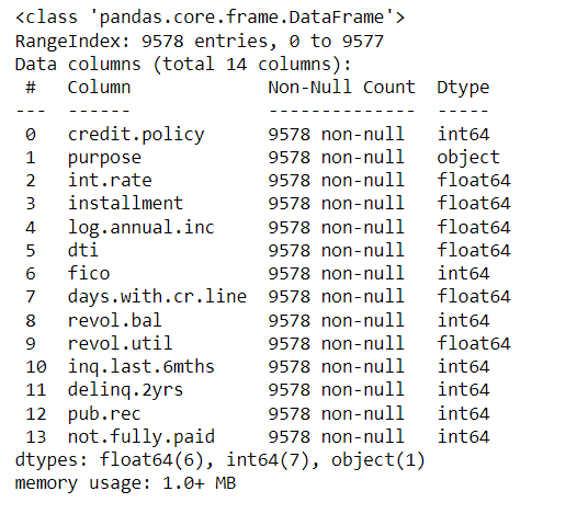
Here, we get the datatypes of all the parameters.
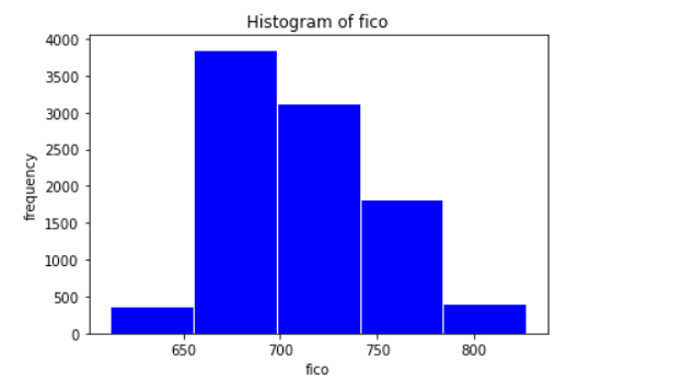
Next, we would do exploratory analysis. In this, we create a histogram of frequency count of fico. FICO is a type of credit score.
plt.hist(data['fico'],color='blue',edgecolor='white',bins=5)
plt.title('Histogram of fico')
plt.xlabel('fico')
plt.ylabel('frequency')
plt.show()
Now, we create a histogram of two FICO distributions against each credit.policy outcome.
plt.figure(figsize=(10,6))
data[data['credit.policy']==1]['fico'].hist(alpha=0.5,color='blue',
bins=30,label='Credit.Policy=1')
data[data['credit.policy']==0]['fico'].hist(alpha=0.5,color='red',
bins=30,label='Credit.Policy=0')
plt.legend()
plt.xlabel('FICO')
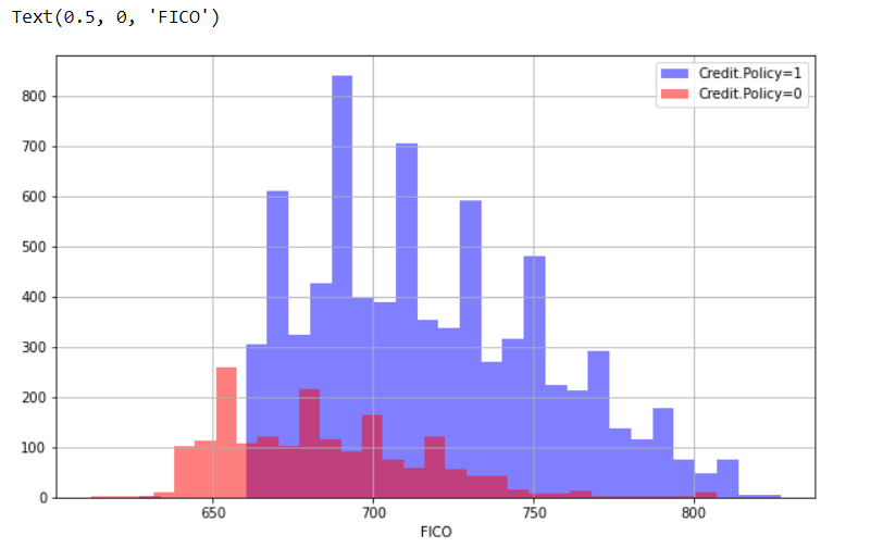
Now, we create a histogram of two FICO distributions against the not.fully.paid column.
plt.figure(figsize=(10,6))
data[data['not.fully.paid']==1]['fico'].hist(alpha=0.5,color='blue',
bins=30,label='not.fully.paid=1')
data[data['not.fully.paid']==0]['fico'].hist(alpha=0.5,color='red',
bins=30,label='not.fully.paid=0')
plt.legend()
plt.xlabel('FICO')
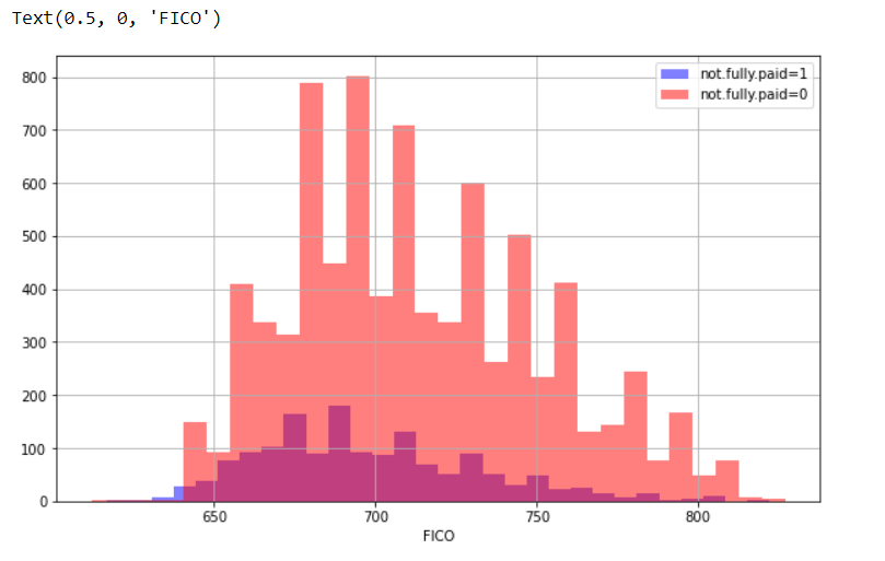
Through histogram we have come to know about the frequency distribution.
Now, we will import the seaborn library and use countplot to show the counts of observations.
import seaborn as sns
plt.figure(figsize=(11,7))
sns.countplot(x='purpose',hue='not.fully.paid',data=data,palette='Set1')
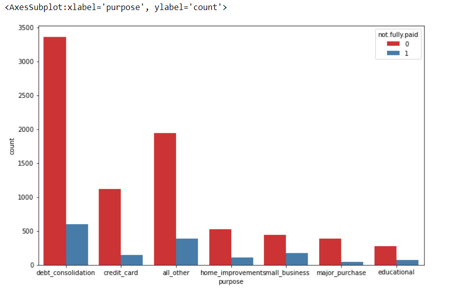
So, above is a countplot showing the counts of loans by purpose where hue=not.fully.paid.
Now, we shall proceed towards data setting by creating a list of elements which will contain the string ‘purpose’ and will be called elements for the sake of convenience. Next, we shall convert categorical data into indicator variables.
Elements=['purpose']
final_data = pd.get_dummies(data,columns=Elements,drop_first=True)
final_data.info()
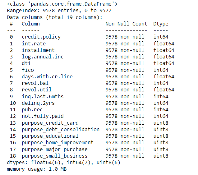
After observing info() of the first dataframe, i.e. data, and the info() of the newly generated dataframe, i.e. final_data, we can see that purpose which was coming under the ‘object dtype’ has been converted to ‘uint8 type’ which is unsigned integer, a 32-bit datum encoding non-negative integers lying in the range of 0 to 4294967295.
Next step would be to perform train-test split by importing train_test_split method from sklearn library.
from sklearn.model_selection import train_test_split
X = final_data.drop('not.fully.paid',axis=1)
y = final_data['not.fully.paid']
X_train, X_test, y_train, y_test = train_test_split(X, y, test_size=0.30, random_state=101)
X would have independent variables, and y would have the target variable. 30% of the dataset would be the testing data. For a deterministic train-test split, random_state is set to an integer value.
from sklearn.tree import DecisionTreeClassifier
dtree = DecisionTreeClassifier()
dtree.fit(X_train,y_train)

In the above lines of code, we are trying to train a decision tree model. So, as a part of the training process we have imported DecisionTreeClassifier, a non-parametric supervised learning method from sklearn library. Next, we create a decision tree classifier and finally, we train it by fitting the model.
predictions = dtree.predict(X_test)
from sklearn.metrics import classification_report,confusion_matrix
print(classification_report(y_test,predictions))

In the above lines of code, classification report, and confusion matrix methods are imported from sklearn. A classification report comprising precision, recall, and f1-score is generated.Next we would generate confusion matrix using cross-tabulation rownames=[‘True’], colnames=[‘Predicted’].
pd.crosstab(y_test, predictions, rownames=['True'], colnames=['Predicted'], margins=True)
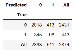
0 indicates the loan was not fully paid whereas 1 indicates the loan was fully paid. Loan not paid was predicted accurately in 2018 subjects and loan fully paid was predicted correctly in 98 subjects. The accuracy of the model using the decision tree is 74%.
We shall try to find out how the random forest model behaved with the same dataset. First, RandomForestClassifier from sklearn would be imported. Next, we create a random forest classifier and finally, we train it by fitting the model.
from sklearn.ensemble import RandomForestClassifier
rfc = RandomForestClassifier(n_estimators=500)
rfc.fit(X_train,y_train)

After training the model, we would finally evaluate the performance of the model following similar procedures similar to the decision tree.
predictions = rfc.predict(X_test)
from sklearn.metrics import classification_report,confusion_matrix
print(classification_report(y_test,predictions))

In the above lines of code, classification report, and confusion matrix methods are imported from sklearn. A classification report comprising precision, recall, and f1-score is generated.Next we would generate confusion matrix using cross-tabulation rownames=[‘True’], colnames=[‘Predicted’].
pd.crosstab(y_test, predictions, rownames=['True'], colnames=['Predicted'], margins=True)
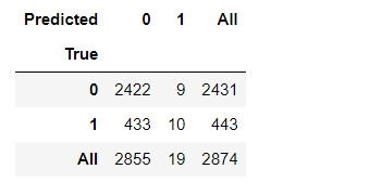
Loan not paid was predicted accurately in 2422 subjects and loan fully paid was predicted correctly in 10 subjects. The accuracy of the model using random forest is 85%.
Conclusion
Decision tree and random forest are important supervised classification tools to predict the outcome of interest. Random forest by virtue of having many decision trees predicts more accurately compared to an individual decision tree. In the given case, the accuracy of the model using random forest was 85% compared to 74% accuracy of the model using the decision tree proving random forest to be a better predictor.
Thank you for your valuable time!


