Plunging into Deep Learning carrying a red wine

This article was published as a part of the Data Science Blogathon

This article would try to address the basic aspects of deep learning. Deep learning attempts to copy the working mechanism of the human brain by combining data inputs, weights, and biases. The basic mechanism of deep learning is to cluster data and make predictions with a high degree of accuracy.

Introduction

Artificial intelligence (AI) is the set, machine learning (ML) is the subset of AI, and deep learning (DL) is the subset of ML which is represented in the image drawn below

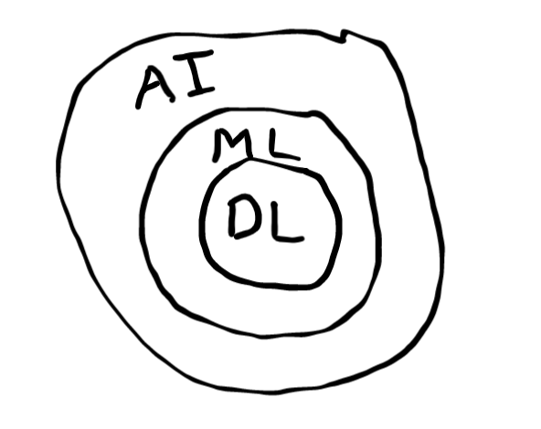
Deep learning involves layers that form a neural network. The layers help in improving accuracy and better prediction. Most of the AI-based applications are extensively driven by DL which range from law enforcement to financial services to the healthcare sector.

Basic Terminologies in deep learning

1) Neuron–

It is the basic component of a neural network. Biologically, a neuron is a system of nerve cells conducting nerve impulses from the receptor to the center. Similarly, in deep learning neurons are the nodes through which the flow of data and computation take place. A neuron is technically a unit of a neural network.

2) Weight–

It is the indicator of the effectiveness of inputs.

3) Bias–

It is an additional parameter equivalent to a constant that enables the adjustment of the output so that model can be fit in the best possible manner for the given dataset.

Let’s understand the relationship among these three terminologies through a diagram

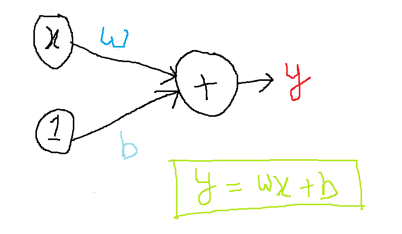
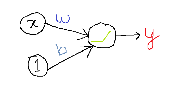
In the above image, x=input; w=weight; b=bias, and y=value of neuron. It is worth mentioning that bias doesn’t have any associated input, for representation purposes we have written ‘1’ so that the exact value of ‘b’ reaches the neuron.
Suppose, we want to know the calorie content of the ’80 cereals’ dataset by training a model with ‘protein’ as input and ‘calories’ as output, we might find the bias, b=90, and weight, w=5. Now, we can calculate the calorie content of the cereal with 4 grams of protein per serving as follows:

Calories = 5*4+90 = 110 

As obvious as stars on a clear night, a dataset will not be limited to one input, on the contrary, there will be many inputs. Let’s observe how multiple units enable model expansion through a diagram

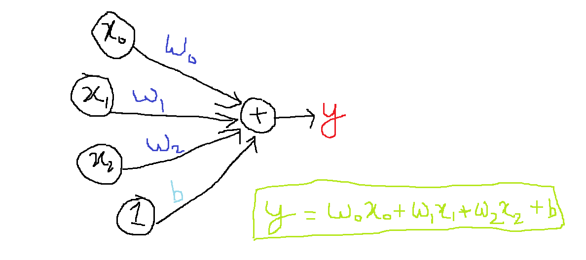
In the above image, we have added more input connections. To obtain the value of output, we have multiplied each input to its connection weight. Finally, we have added all of them together to obtain the output.

Libraries and modules for deep learning

TensorFlow– It is a free and open-source software library used for various tasks with a special focus on deep neural networks.
Keras– It is a library and is open source. For an artificial neural network, it provides a python interface.

Hands-on in deep learning

At the outset, let’s import the library that would be important to read the dataset. After that, we shall load the dataset. The dataset is of red wine quality and the link to the dataset has been given below
Red Wine Quality | Kaggle

import pandas as pd
red_wine = pd.read_csv('winequality-red.csv')
red_wine.head()
red_wine.shape

After loading the dataset, we used the head() function to obtain the first five rows and pertinent columns of the dataset. The shape function is used to find the number of rows and columns. The output has been shown below

There are 1599 rows and 12 columns in the dataset and the name of the columns can be seen through the head() function.
Now, we would try to predict the quality of wine by taking into account various physiochemical measurements. The target is ‘quality’ and the remaining columns are the features that would act as inputs. There are 11 columns.

input_shape=[11]

At this moment we are going to define a linear model. For this, we need to import certain modules and libraries.

from tensorflow import keras
from tensorflow.keras import layers
model =  keras.Sequential([layers.Dense(units=1, input_shape=[11])])

Installation of tensorflow is a prerequisite in Jupyter. For doing this, an anaconda prompt may be opened and a simple command can be given as below to download and install tensorflow

pip install tensorflow

To define a linear model we have imported Keras from tensorflow and layers from tensorflow.keras. Finally, we defined the linear model with 11 inputs and 1 output. Now, Keras is the representative of weights of a neural network with tensor. Tensors are a type of numpy array with the version of TensorFlow. We will obtain the weights of the model defined above.

w, b = model.weights
print("Weightsn{}nnBiasn{}".format(w, b))

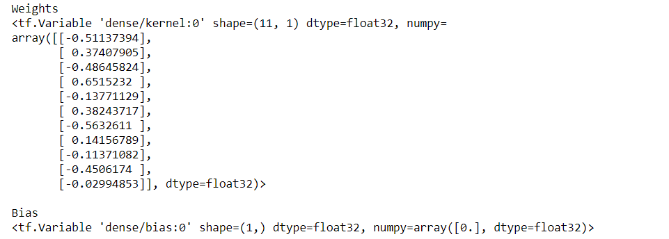
Now, this is an untrained linear model and would be subject to variation. Let’s plot the output of an untrained linear model. Random initialization would produce different results.

import tensorflow as tf
import matplotlib.pyplot as plt
model = keras.Sequential([
    layers.Dense(1, input_shape=[1]),
])
x = tf.linspace(-1.0, 1.0, 100)
y = model.predict(x)
plt.figure(dpi=100)
plt.plot(x, y, 'k')
plt.xlim(-1, 1)
plt.ylim(-1, 1)
plt.xlabel("Input: x")
plt.ylabel("Target y")
w, b = model.weights 
plt.title("Weight: {:0.2f}nBias: {:0.2f}".format(w[0][0], b[0]))
plt.show()

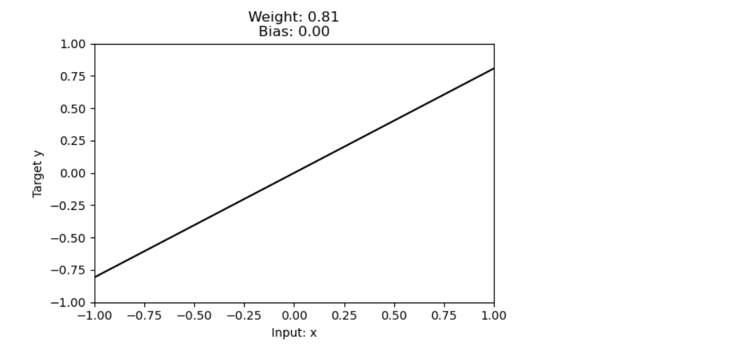
Advancing from a single neuron to a whole neural network

Till now we have focused on a single neuron and its associated function. Now, we will proceed towards a deep neural network.

Concepts associated with deep neural network

1) Layer–

It is a part of the neural network architecture which enables the passage of information from one layer to another. In a neural network, neurons are organized into layers. The collection of several linear units having common inputs lead to the formation of a dense layer. A layer is a kind of data transformation through a neuron.

2) Activation function–

It normalizes the output between -1 and 1 and is a determinant for the relevance of the neuron’s input to the network for prediction. ReLU, elu, selu, and swish are common activation functions with ReLU being the most common. It brings in non-linearity. A representation of ReLU (Rectified linear unit) can be seen in the following diagram

After having some non-linearity, we may think of transforming complex data through stack layers. Let’s try to get a clear picture of this concept through a diagram

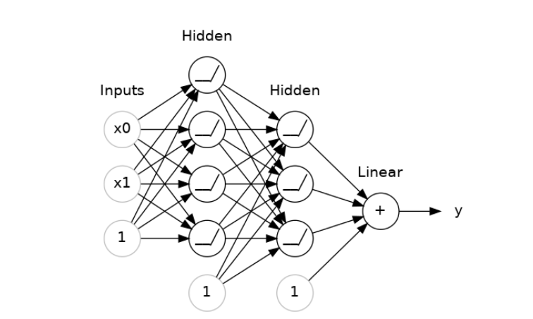
                                                          Image Source: Kaggle

The above image represents a ‘fully connected network’ formed through a stack of dense layers. The layers preceding the output layer are often called the hidden layers as outputs are not explicitly visible.

Sequential models

Lets’ build a model involving layers as inputs and output.

model = keras.Sequential([layers.Dense(units=512,activation='relu',input_shape=[11]),layers.Dense(units=512,activation='relu'),layers.Dense(units=512,activation='relu'),layers.Dense(units=1)])

In the above line of code, we have created a model with 3 hidden layers. All the 3 layers are having 512 units and relu activation. The first layer is having input_Shape as an argument. The output layer has one unit without activation. Let’s have a look at the graph with the following lines of code.

import tensorflow as tf
import matplotlib.pyplot as plt
activation_layer = layers.Activation('relu')
x = tf.linspace(-3.0, 3.0, 100)
y = activation_layer(x) 
plt.figure(dpi=100)
plt.plot(x, y)
plt.xlim(-3, 3)
plt.xlabel("Input")
plt.ylabel("Output")
plt.show()

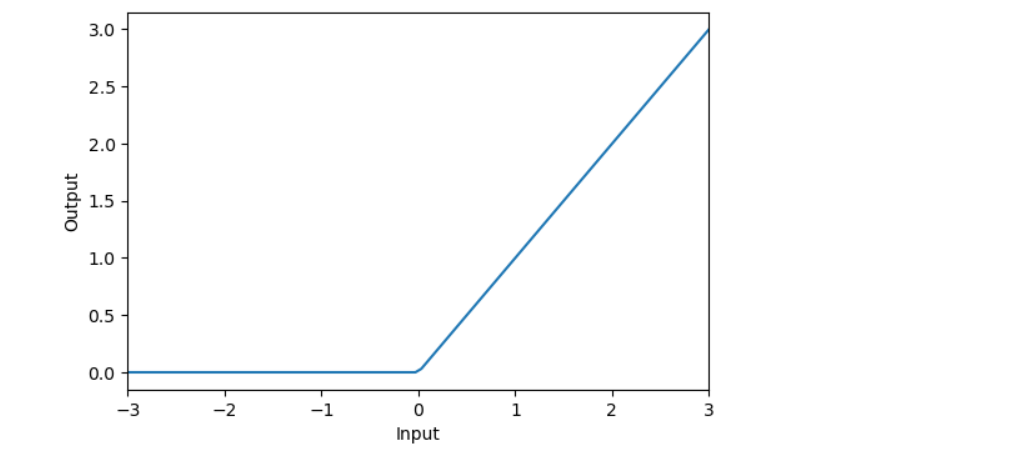
The output is as expected with ReLU activation.

A flight from deep neural networks to SGD
SGD is stochastic gradient descent. Till now we are dealing with an untrained neural network, now we will discuss how to train a neural network.

Key concepts linked with training data

1) Loss function–

It is a measure of the efficiency of prediction about the network. This function measures the difference between the true value of the target and the value model has predicted. MAE(Mean absolute error), MSE(Mean squared error), and Huber loss are some of the loss functions.MAE is the most common loss function for regression problems. It can be better understood as MAE = y_true – y_pred.

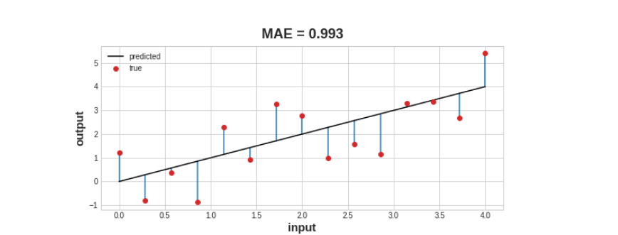
Image Source: Kaggle

2) Optimizer–

SGD is the optimizer. Stochastic means ‘probability’, gradient means ‘vector giving the weights direction’, and descent means ‘towards downside’.It adjusts the weights to minimize the loss. An approach to training is sampling some training data, then running it through the network to make predictions. This step is followed by measuring the loss between the true value and the predicted value. Finally, weights are adjusted to minimize the loss.  Image showing the steps can be seen below

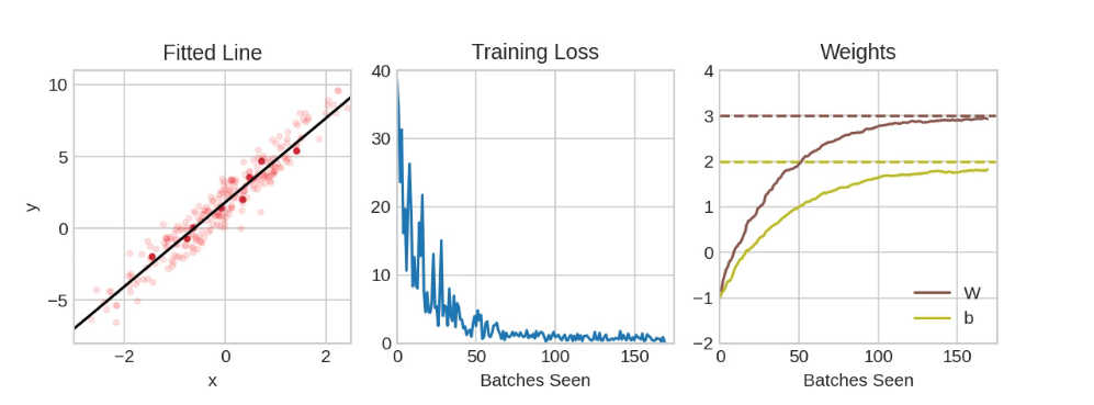
Image Source: Kaggle

3) Epoch–

It refers to a specific period. In deep learning, the sample of training data of each iteration is known as minibatch, complete round of training data is known as an epoch.

4) Learning rate–

It is the determinant of the size of the small shifts that line tends to make in the direction of an individual batch.

Training the model

df_train = red_wine.sample(frac=0.7, random_state=5)
df_valid = red_wine.drop(df_train.index)
display(df_train.head(4))

max_ = df_train.max(axis=0)
min_ = df_train.min(axis=0)
df_train = (df_train - min_) / (max_ - min_)
df_valid = (df_valid - min_) / (max_ - min_)

X_train = df_train.drop('quality', axis=1)

X_valid = df_valid.drop('quality', axis=1)

y_train = df_train['quality']

y_valid = df_valid['quality']

X_train.shape

model = keras.Sequential([
    layers.Dense(512, activation='relu', input_shape=[11]),
    layers.Dense(512, activation='relu'),
    layers.Dense(512, activation='relu'),
    layers.Dense(1),
])

model.compile(
    optimizer='adam',
    loss='mae',
)

history = model.fit(
    X_train, y_train,
    validation_data=(X_valid, y_valid),
    batch_size=256,
    epochs=10,
)

history_df = pd.DataFrame(history.history)
history_df['loss'].plot();

Analysis of the lines of code and the outputs

First of all, we have created validation and training splits. Then, we have rescaled each feature in the range of 0 and 1. Finally, we have split features and the target.
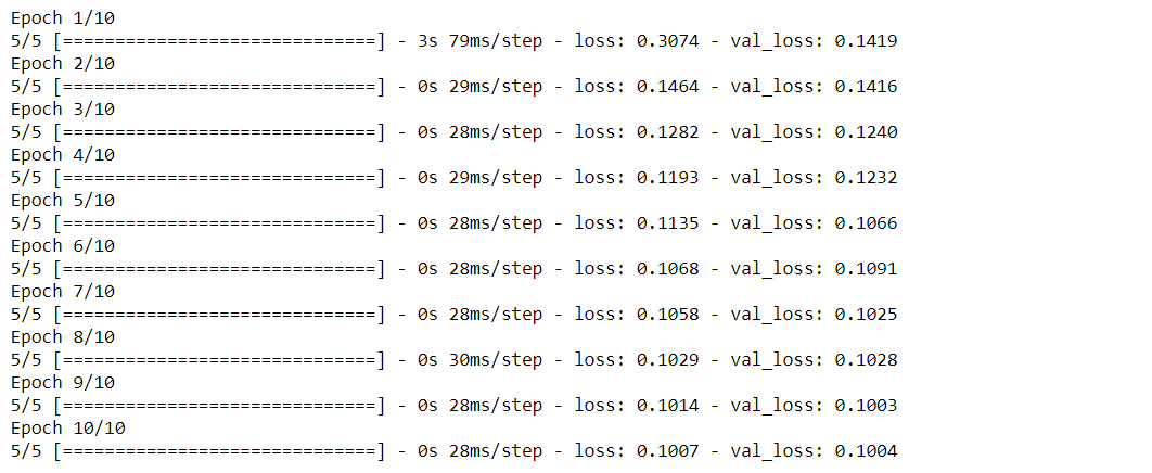
Inputs of the network have been checked through shape function and were found to be 11. The model has been defined by choosing a 3 layer network having neurons>1500. Compilation of the model has been done with the help of ‘Adam’, the optimizer, and ‘MAE’, the loss function. After that training got started with batch size=256 and epochs=10.
From the output, we can observe that the loss approaches a steady state as the number of epochs increases.
A plot is worth a hundred words, so we have tried to plot the pertinent by converting data to a pandas dataframe. It is very important to note remember that the model is not returned by the Keras fit() rather it returns a History.
The output clearly indicates that the loss approaches a steady state as the number of epochs increases and from the graph it can be inferred that the model has learned the needful, so no requirement of additional epochs.

Conclusion

Deep learning can make intelligent decisions on its own much like a human being through neural networks and is the main driving force behind Artificial Intelligence. In this article, most of the basics levels of deep learning have been covered. The follow-up to this article should be to understand overfitting and underfitting, drop-out, batch normalization, and classification.

Thanks a lot for going through this article. I hope that this article did add value to the time you have devoted!

                                                                     References
1. Holbrook, R. (n.d). Kaggle. Intro to Deep Learning. Retrieved from https://www.kaggle.com