This article was published as a part of the Data Science Blogathon
Introduction
The normal distribution is an important class of Statistical Distribution that has a wide range of applications. This distribution applies in most Machine Learning Algorithms and the concept of the Normal Distribution is a must for any Statistician, Machine Learning Engineer, and Data Scientist.
So, In this article, we will explore all the concepts about Normal Distribution in a detailed manner.
Table of Contents
1. What is the Normal distribution?
2. Why is Normal Distribution Important?
3. Parameters of Normal Distribution
- Mean
- Standard Deviation
4. Properties of Normal Distribution
- Symmetricity
- Measures of Central Tendencies are equal
- Empirical Rule
- Skewness and Kurtosis
- The area under the curve
5. Distributions Functions for the Normal Curve
- Probability Density function (PDF)
- Cumulative Density Function (CDF)
6. Applications of Normal Distribution
What is Normal Distribution?
The Normal distribution is also known as Gaussian or Gauss distribution. Many groups follow this type of pattern. That’s why it’s widely used in business, statistics, and in government bodies like the FDA:
- Heights of people.
- Measurement errors.
- Blood pressure.
- Points on a test.
- IQ scores.
- Salaries.
Let’s understand the concept with the help of the following example:
For Example,
The Normal distribution curve is seen in some of the competitive tests like the SAT, UPSC, JEE-Advanced, and GRE, etc. Here the normal distribution indicated that the bulk of students will score the average marks (grade=C), while smaller numbers of students will score the grades (B or D), and a smaller number of students score an F or an A grade.
All these types of inferences are taken from the empirical formula of Normal Distribution, which we will discuss later in this article.
Why is Normal Distribution Important?
There are several reasons why the normal distribution is crucial in statistics. Some of those are as follows:
1. The statistical hypothesis test assumes that the data follows a normal distribution.
2. Both linear and non-linear regression assumes that the residual follows the normal distribution.
3. Moreover, the central limit theorem states that as the sample size increases the distribution of the mean follows normal distribution irrespective of the distribution of the original variable
4. Apart from this most of the statistical software programs support some of the probability functions for normal distribution as well.
Parameters of Normal Distribution
There are two main parameters of a normal distribution- the mean and standard deviation. With the help of these parameters, we can decide the shape and probabilities of the distribution wrt our problem statement. As the parameter value changes, the shape of the distribution changes.
1. Mean
- Researchers used the mean or average value as a measure of central tendency. It can be used to describe the distribution of variables that are measured as ratios or intervals.
- The mean determines the location of the peak, and most of the data points are clustered around the mean in a normal distribution graph.
- If we change the value of the mean, then the curve of normal distribution moves either to the left or right along the X-axis.
Image Source: Google Images
2. Standard Deviation
- The standard deviation measures how the data points are dispersed relative to the mean.
- It determines how far the data points are away from the mean and represents the distance between the mean and the data points.
- The standard deviation defines the width of the graph. As a result, changing the value of standard deviation tightens or expands the width of the distribution along the x-axis.
- Usually, a smaller standard deviation wrt to the mean results in a steep curve while a larger standard deviation results in a flatter curve.
Image Source: Google Images
Properties of Normal Distribution
All forms of the normal distribution share the following characteristics:
1. It is symmetric
- The shape of the normal distribution is perfectly symmetrical.
- This means that the curve of the normal distribution can be divided from the middle and we can produce two equal halves. Moreover, the symmetric shape exists when an equal number of observations lie on each side of the curve.
2. The mean, median, and mode are equal
- The midpoint of normal distribution refers to the point with maximum frequency i.e., it consists of most observations of the variable.
- The midpoint is also the point where all three measures of central tendency fall. These measures are usually equal in a perfectly shaped normal distribution.
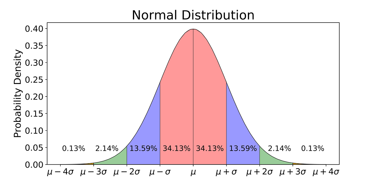
3. Empirical rule
- In normally distributed data, there is a constant proportion of data points lying under the curve between the mean and a specific number of standard deviations from the mean.
- Thus, for a normal distribution, almost all values lie within 3 standard deviations of the mean.
- These check buttons of normal distribution will help you realize the appropriate percentages of the area under the curve.
- Remember that this empirical rule applies to all normal distributions. Also, note that these rules are applied only to the normal distributions.
Fig. Empirical Formula of Normal Distribution
Image Source: Google Images
4. Skewness and kurtosis
- Skewness and kurtosis are coefficients that measure how different the distribution is from a normal distribution.
- It measures the symmetry of the normal distribution while kurtosis measures the thickness of the tail distribution relative to that of normal distribution.
5. Area under the curve
- The total area under the curve is unity(=1)
Distributions Functions for the Normal Curve
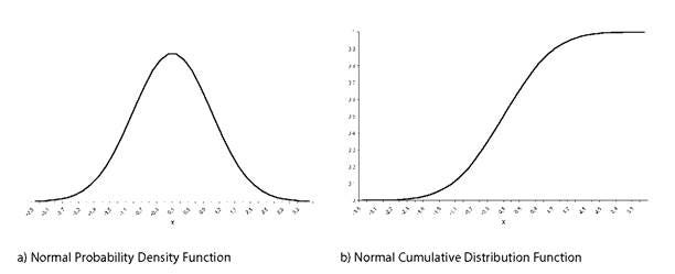
1. Probability Density Function (PDF)
The general formula for the probability density function of the normal distribution is given by,
where,
μ is the location parameter, and
σ is the scale parameter
2. Cumulative Density Function (CDF)
The formula for the cumulative distribution function of the normal distribution is given by,
Remember that the above integral does not exist in a simple closed formula. It is computed numerically.
Fig. PDF and CDF for Normal Distribution
Image Source: Google Images
Special Case:
The case where μ = 0 and σ = 1 is called the standard normal distribution. The equations for the standard normal distribution is
Fig. PDF of Standard Normal Distribution
Applications of Normal Distribution
Let us apply the Empirical Rule to the following problem:
Problem Statement:
Let’s have data of heights of Indian women aged 18 to 24, which is approximately normally distributed with a mean of 65.5 inches and a standard deviation of 2.5 inches.
From the empirical rule, it follows that:
– 68% of these Indian women have heights between 65.5 – 2.5 and 65.5 + 2.5 inches or between 63 and 68 inches,
– 95% of these Indian women have heights between 65.5 – 2(2.5) and 65.5 + 2(2.5) inches, or between 60.5 and 70.5 inches.
– Therefore, the tallest 2.5% of these women are taller than 70.5 inches. (The extreme 5% fall more than two standard deviations, or 5 inches from the mean. And since all normal distributions are symmetric about their mean, half of these women are on the tall side.)
– Almost all young Indian women are between 58 and 73 inches in height if you use the 99.7% calculations.
Endnotes
Thanks for reading!
I hope you enjoyed the article and increased your knowledge about Normal Distribution in Statistics.
Please feel free to contact me on Email
Something not mentioned or want to share your thoughts? Feel free to comment below And I’ll get back to you.
About the Author
Aashi Goyal
Currently, I am pursuing my Bachelor of Technology (B.Tech) in Electronics and Communication Engineering from Guru Jambheshwar University(GJU), Hisar. I am very enthusiastic about Statistics, Machine Learning and Deep Learning.
The media shown in this article are not owned by Analytics Vidhya and are used at the Author’s discretion.


