This article was published as a part of the Data Science Blogathon
Introduction
- Classification algorithms are used to categorize data into a class or category.
- It can be performed on both structured or unstructured data.
- Classification can be of three types: binary classification, multiclass classification, multilabel classification.

Source: https://www.serokell.io
In the above image, you can see that emails are being categorized as spam or not spam. So, it is an example of classification (binary classification).
The algorithms we are going to cover are:
1. Logistic regression
2. Naive Bayes
3. K-Nearest Neighbors
4.Support Vector Machine
5. Decision Tree
We will look at all algorithms with a small code applied on the iris dataset which is used for classification tasks. Dataset has 150 instances(rows), 4 features(columns) and does not contain any null value. There are 3 classes in the iris dataset:
— Iris Setosa
— Iris Versicolour
— Iris Virginica
1. Logistic Regression
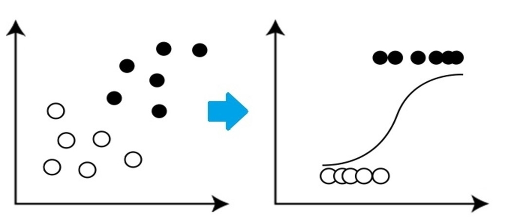
It is a very basic yet important classification algorithm in machine learning that uses one or more independent variables to determine an outcome. Logistic regression tries to find a best-fitting relationship between the dependent variable and a set of independent variables. The best-fitting line in this algorithm looks like S-shape as shown in the figure.

Source: https://www.equiskill.com
Pros:
- It is a very simple and efficient algorithm.
- Low variance.
- Provides probability score for observations.
Cons:
- Bad at handling a large number of categorical features.
- It assumes that the data is free of missing values and predictors are independent of each other.
Example:
2. Naive Bayes
Naive Bayes is based on Bayes’s theorem which gives an assumption of independence among predictors. This classifier assumes that the presence of a particular feature in a class is not related to the presence of any other
feature/variable.
Naive Bayes Classifier are of three types: Multinomial Naive Bayes, Bernoulli Naive Bayes, Gaussian Naive Bayes.
Pros:
- This algorithm works very fast.
- It can also be used to solve multi-class prediction problems as it’s quite useful with them.
- This classifier performs better than other models with less training data if the assumption of independence of features holds.
Cons:
- It assumes
that all the features are independent. While it might sound great in
theory, but in real life, anyone can hardly find a set of independent features.
Example:from sklearn.datasets import load_iris from sklearn.model_selection import train_test_split from sklearn.naive_bayes import GaussianNB X, y = load_iris(return_X_y=True) X_train, X_test, y_train, y_test = train_test_split(X, y, test_size=0.25, random_state=142) Naive_Bayes = GaussianNB() Naive_Bayes.fit(X_train, y_train) prediction_results = Naive_Bayes.predict(X_test) print(prediction_results)
Output:array([0, 1, 1, 2, 1, 1, 0, 0, 2, 1, 1, 1, 2, 0, 1, 0, 2, 1, 1, 2, 2, 1,0, 1, 2, 1, 2, 2, 0, 1, 2, 1, 2, 1, 2, 2, 1, 2]) These are the classes predicted for X_test data by our naive Bayes model.
3. K-Nearest Neighbor Algorithm
You must have heard of a popular saying:
“Birds of a feather flock together.”
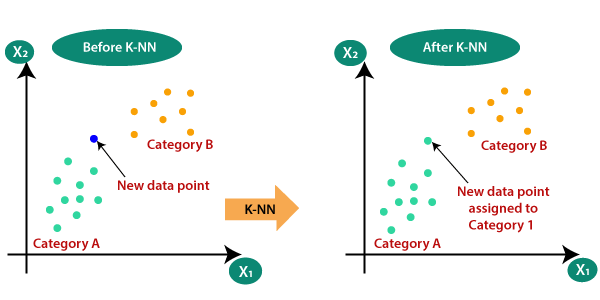
KNN works on the very same principle. It classifies the new data points depending upon the class of the majority of data points amongst the K neighbor, where K is the number of neighbors to be considered. KNN captures the idea of similarity (sometimes called distance,
proximity, or closeness) with some basic mathematical distance formulas like euclidean distance, Manhattan distance, etc.

Source: https://www.javatpoint.com
Choosing the right value for K
To select the K that’s right for the data you want to train, run the KNN algorithm several times with different values of K and choose that value of K which reduces the number of errors on unseen data.
Pros:
- KNN is simple and easiest to implement.
- There’s no need to build a model, tuning several parameters, or make additional assumptions like some of the other classification algorithms.
- It can be used for classification, regression, and search. So, it is flexible.
Cons:
- The algorithm gets significantly slower as the number of examples and/or predictors/independent variables increase.
Example:from sklearn.neighbors import KNeighborsClassifier X_train, X_test, y_train, y_test = train_test_split(X, y, test_size=0.25, random_state=142) knn = KNeighborsClassifier(n_neighbors=3) knn.fit(X_train, y_train) prediction_results = knn.predict(X_test[:5,:) print(prediction_results)
Output:array([0, 1, 1, 2, 1]) We predicted our results for 5 sample rows. Hence we have 5 results in array.
4. SVM
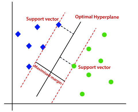
SVM stands for Support Vector Machine. This is a supervised machine learning algorithm that is very often used for both classification and regression challenges. However, it is mostly used in classification problems. The basic concept of the Support Vector Machine and how it works can be best understood by this simple example. So, just imagine you have two tags: green and blue, and our data has two features: x and y. We want a classifier that, given a pair of (x,y) coordinates, outputs if it’s either green or blue. Plot labeled training data on a plane and then try to find a plane (hyperplane of dimensions increases) that segregates data points of both colors very clearly.

Source: https://www.javatpoint.com
But this is the case with data that is linear. But what if data is non-linear, then it uses kernel trick. So, to handle this we increase dimension, this brings data in space and now data becomes linearly separable in two groups.
Pros:
- SVM works relatively well when there is a clear margin of separation between classes.
- SVM is more effective in high-dimensional spaces.
Cons:
- SVM is not suitable for large data sets.
- SVM does not perform very well when the data set has more noise i.e. when target classes are overlapping. So, it needs to be handled.
Example:from sklearn import svm svm_clf = svm.SVC() X_train, X_test, y_train, y_test = train_test_split(X, y, test_size=0.25, random_state=142) svm_clf.fit(X_train, y_train) prediction_results = svm_clf.predict(X_test[:7,:]) print(prediction_results)
Output:array([0, 1, 1, 2, 1, 1, 0])
5.Decision Tree
The decision tree is one of the most popular machine learning algorithms used. They are used for both classification and regression problems. Decision trees mimic human-level thinking so it’s so simple to understand the data and make some good intuitions and interpretations. They actually make you see the logic for the data to interpret. Decision trees are not like black-box algorithms like SVM, Neural Networks, etc.
Source: https://www.aitimejournal.com
For example, if we are classifying a person as fit or unfit then the decision tree looks like somewhat this above in the image.
So, in short, a decision tree is a tree where each node represents a
feature/attribute, each branch represents a decision, a rule, and each leaf represents an outcome. This outcome may be categorical or continuous value. Categorical in case of classification and continuous in case of regression applications.
Pros:
- When compared to other algorithms, decision trees require less effort for data preparation while pre-processing.
- They do not require normalization of data and scaling as well.
- Model made on decision tree is very intuitive and easy to explain to technical teams as well as to stakeholders also.
Cons:
- If even a small change is done in the data, that can lead to a large change in the structure of the decision tree causing instability.
- Sometimes calculation can go far more complex compared to other algorithms.
- Decision trees often take higher time to train the model.
Example:from sklearn import tree dtc = tree.DecisionTreeClassifier() X_train, X_test, y_train, y_test = train_test_split(X, y, test_size=0.25, random_state=142) dtc.fit(X_train, y_train) prediction_results = dtc.predict(X_test[:7,:]) print(prediction_results)
Output:array([0, 1, 1, 2, 1, 1, 0])
Conclusion
In summary, these classification algorithms present varied strengths for diverse data situations. Each algorithm has its merits, from the straightforward nature of Logistic Regression to the adaptability of K-Nearest Neighbors and the robustness of Decision Trees. Exploring these methods lays the foundation for mastering machine learning and comprehending the intricacies of predictive modeling.
These are the popular 5 classification algorithms, there are many more and advanced algorithms too. Explore them as well. Let’s connect on LinkedIn
Thanks for reading if you reached here 🙂
FAQs
There are many different classification algorithms used in data mining, each with its own strengths and weaknesses. Some of the most popular algorithms include decision trees, logistic regression, naive Bayes classification, k-nearest neighbors, and support vector machines. The choice of which classification algorithm to use depends on the specific task at hand.
Classification algorithms are essential tools in machine learning, enabling the categorization of data points into predefined classes. They are employed in a wide range of applications, including spam filtering, medical diagnosis, and customer segmentation. Several popular classification algorithms exist, each with its own strengths and limitations. The choice of algorithm depends on the specific task, data characteristics, and computational resources available.
Classification algorithms in image processing categorize images into predefined classes, employing supervised or unsupervised learning techniques. Supervised algorithms use labeled training data, while unsupervised algorithms discover patterns from unlabeled data. Common algorithms include Support Vector Machines (SVMs), K-Nearest Neighbors (KNN), and neural networks. Applications span medical diagnosis, object detection, and scene understanding.
The media shown in this article are not owned by Analytics Vidhya and is used at the Author’s discretion.


