This article was published as a part of the Data Science Blogathon.
Introduction
Have you ever been in a situation, where you were not sure about which metric to apply to evaluate your models? These situations can be tackled by understanding the use-case of each metric.
Everyone knows the basic know-how of all frequently used classification metrics but when it comes to knowing the right one to use to evaluate the performance of their classification model, very few are confident in the next step to take.
Supervised learning normally falls either under regression (having continuous targets) or under classification (having discrete targets). However, in this article, I will try to focus on a very little yet very important part of machine learning, which being a favorite topic of interviewers – “who knows what”, can also help you get your concepts right on classification models and eventually on any business problem. This article will help you learn that when someone tells you that an ml model is giving 94% accuracy, what questions you should ask to know if the model is actually performing as required.
So how to decide on the questions that will help?
Now, that’s a thought for the soul.
We will answer that by knowing how to evaluate a classification model, the right way.
We will go through the below topics in this article:
-
Accuracy
-
Shortcomings
-
Confusion Matrix
-
Metrics based on the Confusion matrix
-
Recap
After reading this article you will have the knowledge on:
-
What is the confusion matrix and why you need to use it?
-
How to calculate a confusion matrix for a 2-class classification problem
-
Metrics based on confusion matrix and how to use them
Accuracy and its shortcomings:
Accuracy (ACC) measures the fraction of correct predictions. It is defined as “the ratio of correct predictions to total predictions made”.
Problem with accuracy:
It hides the detail you need to better understand the performance of your classification model. You can go through the below examples that will help you understand the problem:
-
Multi-class target variable: When your data has more than 2 classes. With 3 or more classes you may get a classification accuracy of 80%, but you don’t know if that is because all classes are being predicted equally well or whether one or two classes are being neglected by the model.
-
Imbalanced dataset: When you have imbalanced data (does not have an even number of classes). You may achieve an accuracy of 95% or more but is not a good score if 95 records for every 100 belong to one class as you can achieve this score by always predicting the most common class value. Example dataset – Breast cancer dataset, spam vs not spam dataset.
A typical example of imbalanced data is encountered in an e-mail classification problem where emails are classified into spam or not spam. Here, the count of spam emails is considerably very low (less than 10%) than the number of relevant (not spam) emails (more than 90%). So, the original distribution of two classes leads to an imbalanced dataset.
If we take two classes, then balanced data would mean that we have 50% points for each of the classes. Also, if there are 60-65% points for one class and 40% for the other class, it should not cause any significant performance degradation, as the majority of machine learning techniques can handle little data imbalance. Only when the class imbalance is high, e.g. 90% points for one class and 10% for the other, Accuracy and few other optimization measures may not be as effective and would need modification.
Classification accuracy does not bring out the detail you need to diagnose the performance of your model. This can be brought out by using a confusion matrix.

Confusion Matrix:
Wikipedia defines the term as “a confusion matrix, also known as an error matrix is a specific table layout that allows visualization of the performance of an algorithm”.

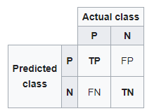
A confusion matrix for two classes (+, -) is shown below.
There are four quadrants in the confusion matrix, which are symbolized as below.

confusion matrix
- True Positive (TP): The number of instances that were positive (+) and correctly classified as positive (+v).
- You predicted a mail is a spam and it actually is.
- False Negative (FN): The number of instances that were positive (+) and incorrectly classified as negative (-). It is also known as Type 2 Error.
- You predicted a mail is not spam and it actually is.
- True Negative (TN): The number of instances that were negative (-) and correctly classified as (-).
- You predicted a mail is not spam and it actually is not.
- False Positive (FP): The number of instances that were negative (-) and incorrectly classified as (+). This also known as Type 1 Error.
- You predicted a mail is not spam and it actually is.
To add a little clarity:
Upper Left: True Positives for correctly predicted event values.
Upper RIght: False Positives for incorrectly predicted event values.
Lower Left: False Negatives for correctly predicted no-event values.
Lower Right: True Negatives for incorrectly predicted no-event values.
Metrics based on Confusion matrix:
-
Precision
-
Recall
-
F1-Score
Precision
Precision calculates the ability of a classifier to not label a true negative observation as positive.
Precision=TP/(TP+FP)
Using Precision
We use precision when you are working on a model similar to the spam detection dataset as Recall actually calculates how many of the Actual Positives our model capture by labeling it as Positive.
Recall (Sensitivity)
Recall calculates the ability of a classifier to find positive observations in the dataset. If you wanted to be certain to find all positive observations, you could maximize recall.
Recall=TP/(TP+FN)
Using Recall
We always tend to use the recall, when we need to correctly identify the positive scenarios, like in a cancer detection dataset or a fraud detection case. Accuracy or precision won’t be that helpful here.
F-measure
In order to compare any two models, we use F1-Score. It is difficult to compare two models with low precision and high recall or vice versa. F1-score helps to measure Recall and Precision at the same time. It uses Harmonic Mean in place of Arithmetic Mean by punishing the extreme values more.
Understanding the Confusion Matrix
Let’s say we have a binary classification problem where we want to predict if a patient has cancer or not, based upon the symptoms (the features) fed into the machine learning model (classifier).
As studied above, the left-hand side of the confusion matrix shows the class predicted by the classifier. Meanwhile, the top row of the matrix shows the actual class labels of the examples.
If the problem set has more than two classes, the confusion matrix just grows by the respective number of classes. For instance, if there are four classes it would be a 4 x 4 matrix.
In simple words, no matter the number of classes, the principal will remain the same: The left-hand side of the matrix is the predicted values, and the top the actual values. What we need to check is where they intersect to see the number of predicted examples for any given class against the actual number of examples for that class.
While you could manually calculate metrics like confusion matrix, precision, and recall, most machine learning libraries, such as Scikit-learn for Python, have built-in methods to get these metrics.
Generating A Confusion Matrix In Scikit Learn
We have already covered the theory on working of the confusion matrix, here we will share the python commands to get the output of any classifier as a matrix.
To get the confusion matrix for our classifier, we need to create an instance of the confusion matrix we imported from Sklearn and pass it the relevant arguments: the true values and our predictions.
from sklearn.metrics import confusion_matrix
c_matrix = confusion_matrx(y_test, predictions)
print(c_matrix)
Recap
In a brief recap, we looked into:
-
accuracy
-
problems it can bring to the table
-
confusion matrix to better understand the classification model
-
precision and recall and scenario on where to use them
We lean towards using accuracy because everyone has an idea of what it means. There is a need to increase the use of better-suited metrics such as recall and precision which may seem foreign. You now have an intuitive sense of why these work better for some problems such as imbalanced classification tasks.
Statistics provide us with formal definitions to evaluate these measures. Our job as a data scientist is about knowing the right tools for the right job, and this brings in the need to go beyond accuracy when working with classification models.
Using recall, precision, and F1-score (harmonic mean of precision and recall) allows us to assess classification models and also makes us think about using only the accuracy of a model, especially for imbalanced problems. As we have learned, accuracy is not a useful assessment tool on various problems, so, let’s deploy other measures added to our arsenal to assess the model!
Rohit Pant


