This article was published as a part of the Data Science Blogathon.
Introduction
I have been thinking of writing something related to Recurrent Neural Networks but since there are a lot of blog posts already available I just held myself from doing the repetitive work until now when I thought of reviewing a research paper and then adding some additional information to it so that new readers will find it fascinating.
So starting with a question which I always do :), why we need RNNs while we had Feed Forward and Convolutional Neural Networks? It turns out Feed-Forward Networks are pretty good with sequential data while Convolutional Neural Networks are with images when it comes to temporal dependency (dependency over time) these networks fail that’s the reason we don’t usually use ANNs or CNNs for tasks like speech synthesis, music generation, text generation, etc.
Similar tasks like speech recognition, stock price predictions, language translation, etc are time-variant so we required to have a model which have some memory component to consider time. The first attempt to add memory in the neural networks was Time Delay Neural Networks (TDNNs) which were designed to take inputs from past time stamps but failed for a disadvantage which was, these networks were limited to the window size chosen (number of past time stamps).
Next was Elman Networks or Jordan Networks currently referred to as RNN (Recurrent Neural Networks). These two models suffered from a vanishing gradient problem in which the contribution of information becomes lesser and lesser over time. In the early 90s, LSTMs (Long Short Term Memory Networks) was introduced to address this problem by using the concept of gates, one variation to these is often referred to as GRUs (Gated Recurrent Units) which are now widely popular as one type of RNN. So with this short description, we are now clear with RNNs and their types.
Traditional neural networks tend that each data point contributes only once as the network trains and after training the state of it lost, which is not a good shot for data having time dependency. while RNNs tend to consider a window of data and train models according to that.
Some of the important questions which I had about RNNs were as follows-
1. Why sequentially matters?
There are a lot of real-life scenarios like image processing, voice recognition, language translations in which sequence matters. For example, If I write “are you how ?” will it make sense? no right because our brain is trained to process this sentence in sequence. One more example for this would be video processing, what if you are watching the world-famous movie Avengers: Endgame and the climax one where Ironman dies ( pretty sad for all the fans including me ) is shown to you first that would be of no sense also somewhat disappointing.
That is because we have trained our brain with this sequenced information and some change in their order would make it hogwash. Similarly, these tasks need a model that considers time, traditional models like SVM, logistic regression, or Neural Networks like FFN are not capable of doing these tasks. While talking about AI/ML, the primary conception of Artificial Intelligence is a machine that can engage with a human in a way similar to other humans.
One of the greatest minds, Alan Turing has mentioned in his paper “Computing Machinery and Intelligence” that Artificial Intelligence is the ability of a machine to convincingly engage in dialogue ( what we will call an AI-based advanced chatbot ), this will be only done when computers will be able to process the time-dependent data in the same way as the human mind does. With that, I hope you are a little clear about why we are focusing on the term sentimentality.
2. Why having another model while we have Markov Models?
Markov models are also capable of representing temporal dependencies. These models explain the transition of states in an observed sequence. In standard Markov models current state is dependent on the last one state which can be extended to a particular window say 5 or 10, but increasing the context window also increases the state-space complexity of the model which makes them impractical for modeling in a long context window.
This is the limitation that makes Markov models less suitable for time-dependent tasks with the long context window and enables RNNs to solve the problem.
For a better understanding of RNNs, we need to first understand the FFNN ( Feed Forward Neural Networks ) and Backpropagation.
FFNN ( Feed Forward Neural Networks ) and Backpropagation:
The idea of a Neural Network came from the biological structure of the human brain. Similar to the brain, Neural Network has multiple neurons referred to as nodes or units which are connected through the synapses called edges, these nodes transfer data using the synapses. Each node in the network has some kind of activation function associated with it which introduces nonlinearity in the network, and each edge has some weight value associated with it which generally ranges between 0–1.
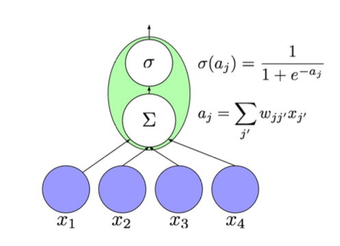
For mathematical representation lets consider activation function associated with the node j is lj and Associated with each edge from node j′ to j is a weight wjj′ then the value vj of each neuron j is calculated by applying its activation function to the sum of the product of the input vector vj’ and weights matrix wjj’.

where vj’ is the output of the node j’.

Figure 1.2 shows the flow of calculation, each input (x1, x2, x3, x4 ) is multiplied with their corresponding edge weights and sum together to apply the activation function on it to introduce the nonlinearity.
When I first studied Neural Networks I had the question that in the human brain neurons are unordered they are just randomly connected and if we are gonna mimic that how the computations are going to take place, the answer to this was FFNN where nodes can be arranged in multiple layers. FFNN has a single input layer and a single output layer and all other layers in between are referred to as hidden layers, each layer takes input from its previous layer.
FFNN can be simulated as nonlinear function approximation ( in general consider is at an umbrella trying to cover something or in actual terms trying to fit a function between input data points such that for new input a new output is generated ) which tries to minimize the error between the actual values and the predicted values.

Here x̅ is the input vector and W is a weights matrix, which is used to calculate the predicted value ȳ. While talking about the actual working of NN the inputs ( x ) are passed to the input layer of the network which is then multiplied with weights and then summed together to have a single linear value which is when passed to an activation function to convert it into nonlinear, this process continues until we reach the output layer which is desired output.
Our goal here is to find the optimal weights for each edge in the network that minimizes the loss(error difference between actual and predicted values)
For keeping loss at a minimum we need to iteratively update the weights of the network, but how we can do it when we are using FFNN which is just calculating the difference of actual and predicted values? This is where backpropagation comes into play when an error is calculated using FFNN, backpropagation is applied to the network to change the weights of the network by backtracking it and this process repeats until we find optimal weights.
For understanding the maths behind FFNN and backpropagation you can check this awesome blog:
so now back to RNN, how these FFNN and backpropagation concepts are used in RNN.
Recurrent Neural Networks
RNNs are based on the same principles as FFNN, except the thing that it also takes care of temporal dependencies by which I mean, in RNNs along with the input of the current stage, the previous stage’s input also comes into play, and also it includes feedback and memory elements. Or we can say that RNN output is the function of current as well as previous inputs and the weights.

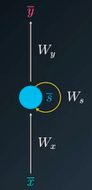
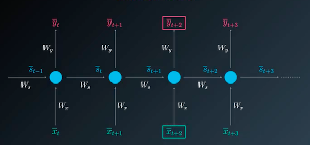
Figure 1.4 shows the basic structure of RNN, this is referred to as the folded RNN model. where x̅ and ȳ represent the input and the output respectively, s represents the states which is generally previous input, and Wx, Ws, Wy represents the weights for input, hidden and output layers respectively. When we unfold the following model it will look like this:

Now you can clearly see each node is having two inputs, current ( represented using x̅ ) and previous ( represented using st ) and produce some output. In FFNN we obtain the input for the hidden layer by applying the activation function, for this, we only need the input vector and the weights matrix.

RNNs also use activation functions only with a small change:

The hidden layer’s input is calculated using the sum of the product of input and state vectors with their respective weights matrix. and output is calculated the same in both FFNNs and RNNs using the following formula:

The unfolded architecture of the RNNs can be altered as per the requirement, say if you want to do the sentiment classification task we can have multiple inputs and single output while in the case of language generation models we need to have multiple inputs and multiple outputs, also RNNs can be stacked together for some special use cases.
Feed Forward process as we have seen is almost the same in both FFNNs and RNNs, but when we talk about Back-propagation in RNNs it is often referred to as Back-propagation Through Time ( BPTT ) which is dependent on previous states.
Training Recurrent Neural Networks
Training RNNs is considered to be difficult, in order to preserve long-range dependencies it often meets one of the problems called Exploding Gradients ( weights become too large that over-fits the model ) or Vanishing Gradients ( weights become too small that under-fits the model ). The occurrence of these two problems depends on the activation functions used in the hidden layer, with the sigmoid activation function vanishing gradient problem sounds reasonable while with rectified linear unit exploding gradient make sense.
For these problems, a concept called regularisation is used which helps to tackle both vanishing and exploding gradient. RNNs can be easily trained using some Deep Learning libraries like Tensorflow, PyTorch, Theano, etc. The only important thing here is if you want to run RNNs, GPUs are needed since they are deeper networks for smaller networks you can make use of online GPU enabled notebooks like Google Colab, Kaggle Kernels, etc.
As an extension to RNNs, LSTMs ( Long Short Term Memory ) and BRNNs ( Bidirectional Recurrent Neural Networks ) were proposed which I will discuss in the next article.
References:
1. A Critical Review of Recurrent Neural Networks for Sequence Learning: https://arxiv.org/abs/1506.00019
2. Udacity Deep Learning: https://www.udacity.com/
Thanks for reading this article do like if you have learned something new, feel free to comment See you next time !!! ❤️


