Introduction
Machine learning and Artificial Intelligence developments are happening at breakneck speed! At such pace, you need to understand the developments at multiple levels – you obviously need to understand the underlying tools and techniques, but you also need to develop an intuitive understanding of what is happening.
By the end of this article, you will develop an intuitive understanding of RNNs, especially LSTM & GRU.
Ready? Let’s go!
Table of Contents
- Simple exercise – Tweet classification
- How does our brain process the English language?
- Notations in this article
- Let’s start with RNN
- Consider Gated Recurrent Unit (GTU) first
- Understanding Long Short Term Memory (LSTM)
- A short note on Bidirectional RNN
- LSTM v GRU – who wins?
Let’s start with a simple exercise – tweet classification
Have a look at this article on NLP. I took a handful of tweets and used the word count of positive versus negative words to classify the sentiment of the tweet.
This approach might work for simple sentences but will fail in the case of long sentences with mixed emotions or negated phrases like “not at all happy”.
Any thoughts on why this approach fails?
The answer is simple. The algorithm is far from how humans evaluate a sentiment score. Let me elaborate further. Consider the below sentence:
I have a bank account in TD bank which is neither the best nor the largest in US but the quality of service I get is exceptional.
Anyone can make out that the sentiment of this sentence is positive. But an n-gram scoring algorithm, solely based on word/phrase counting, gets confused because the sentence starts with a double negative and finally finds one positive to end the sentence. Analyzing each word, or a group of words individually, does no justice to the meaning of the sentence.
Before we talk about sophisticated tools like RNN, LSTM and GRU, let’s first develop an intuition of what do we expect these models to do by understanding how the human brain really processes written/spoken language.
How does our brain process the English Language?
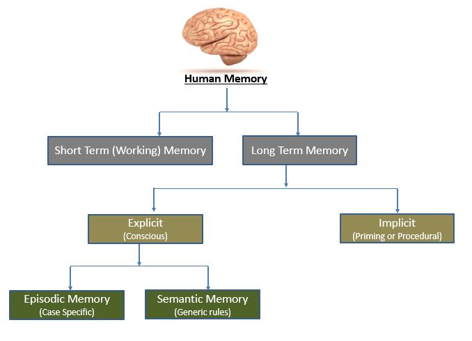
Don’t worry, this is not a biology lesson. We are only interested in understanding how our brain stores all the information it gets from all sensory organs. Following is a simplistic view of how humans store data:
Read this statement – “Bitcoin peaked in Dec 2017 to a value of $19,870.62 but dropped down steeply to a range of $6000-$7000. The current value of Bitcoin is about $6635.38”.
If I ask you a question right now – “What is the current value of Bitcoin?”, it is highly likely that you will reply “$6635.38”. However, if I ask you this question tomorrow, it’s highly likely that your answer will be in a range, something like – “$6000 – $7000”. The reason we tend to forget precise values over time is because we initially retrieve the information from short term memory and later from long term memory.
Our short term memory is like a scratch pad and our brain uses gates to find relevant concepts that need to be retained in our long term memory. Implicit memory is responsible for unconscious activities like riding bicycle or putting on shoes, etc. Explicit memory is the conscious memory and comprises of Episodic Memory and Semantic Memory. Episodic is a very case specific learning we do, for instance – your last trip to a beach or your memories of schooling etc. Semantic is generic rules we learn over time, like – snakes are poisonous or the Earth is round, etc.
Now let’s narrow down the discuss to NLP. If you are reading a novel, say “Julius Caesar”, you do not register each and every line that is written to your short-term memory but you will learn and store the generic style of writing/grammar in your Semantic Memory, and learn about characters like Caesar/Brutus and important events in our Episodic memory. If we want to build a neural network that can compete with humans in terms of Natural Language Understanding, it needs to do exactly the same, i.e., use short term memory to register everything that it reads, use gates to identify what do we need in long term memory, and finally a long term memory to create something like a knowledge graph.
Recurrent Neural Networks (RNNs) do exactly those things to understand natural language or any other sequential data. Long Short Term Memory (LSTM) and Gated Recurrent Unit (GRU) are two special architectures of RNN that are great tools to have in your kit when trying to understand the semantics of a language. Now that you understand what this new architecture does, we will now look at how they perform exactly as the human brain does (or close enough).
Notation we will use in this article
Here is a sample problem to define our notation – you have 1000 tweets on Cryptocurrency and you are tasked with identifying the cryptocurrency that is being most talked about. Here are couple of sample tweets :
Tweet 1 : Feeling bullish about Bitcoin. Last I saw Bitcoin going strong was in Dec 2017.

Tweet 2: Both Ether and Litecoin are going to take over BTC. BTC is too slow and expensive.
Notice that a single coin can be referred to in multiple ways – Bitcoin or BTC or something else. You want to train a neural network that can identify the occurrence of coin names. One way to define output sequence is as follows (Replace irrelevant words with “U” and coin name by their ticker):
Tweet 1 (output) : U U U BTC U U U BTC U U U U U. (I have removed numeric and full stops and simply replaced all Bitcoin references with BTC and rest as U.

Tweet 2 (output) : U ETH U LTC U U U U U BTC BTC U U U U U
Our inputs will be denoted as X <i> (j) where i is the word number in the sequence and j is the sequence number. For instance, “bullish” is X <2> (1), “Both” is X <1> (2). Similarly, Y <1> (2) is “U” and Y<4> (1) is “BTC”. Try to memorize these notations as we’ll reference them later in this article. We will denote W and C to identify weights and biases in all equations and drop subscripts for simplicity.
We will also refer to two types of main functions in our RNNs –
- Squashing function which compresses the score to a range (-1, 1). Tanh is one of the most popular squashing functions.
- Activation function which converts our score to probabilities with range (0,1). Sigmoid or Softmax can be used as an activation function.
Let’s start with RNN
Why do we need a special type of neural network at all for NLP based problems?
Here are a few (not exhaustive) reasons why simple a neural net cannot do well on NLP problems:
- Simple neural network will need a fixed length of input sequence, which is not true for texts. This is a minor challenge as we can pad all sequences by 0s but such intervention increases redundancy.
- Simple neural network will have enormous number of parameters to train. For instance, if our individual sequence has 20 elements and our vocabulary is of 10k words, our input feature list becomes 200k long.
- Simple neural network does not have shared weights over sequences. If you have read about CNN, you will know how shared weights in the convolution layer helps us to compensate for spatial movement of the subject. Similarly, if our words of key interest move in the sequence, it should have minimal impact to our model.
- Additionally, our model should try to understand the meaning of a sentence as a whole instead of individual words. This is exactly what LSTM and GRU, which are types of RNN, do.
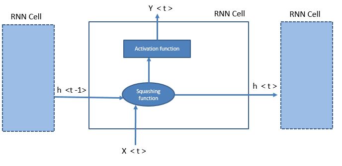
Following is a pictorial view of a single RNN:
The blue outlines are individual RNN cells. I have collapsed the first and third cell for simplicity. Each RNN cell gets a hidden state from the previous RNN and a new input element. It then generates an output and passes on the modified hidden state.
So for a sequence of 10 elements in a series, you will have 10 units modifying the hidden state, which is trying to capture the semantic of the sentence. Now this hidden state, which has all the information in the form of numbers, can be used directly to understand the sentiment of the sentence or any other information. Notice that instead of using individual words to understand the meaning of a sentence, we are now working more human like, i.e., creating a vector that has all the stored information of the entire sentence in a compressed form.
The Squashing function will look something like:
h <t> = tanh(W * (X <t>,h<t-1> ) + C)
So, we found a jackpot to crack any NLP problem. But we have two major problems in this architecture. First, the vanishing gradient and, second, the exploding gradient. In the last 5 years we have solved both these problems in vastly different ways. The solution to exploding gradient is simple – just define a ceiling for the gradient. But the solution for vanishing gradient challenge is a much more involved process. Let’s try to understand what Vanishing gradient really does to our algorithm. Consider this sentence:
My wife, who loves to play with dogs, ______ (hate or hates) cats.
We want our neural network to fill in the blank. The actual subject “wife” will take the verb “hates” but this subject is far away from our verb. The English language can give grammatical tasks that are much more complex but are critical in understanding the meaning of the sentence. Neural Networks suffering with vanishing gradient problem tend to miss out relations between words that are far away from each other. LSTM and GRU are the architects of RNN that can solve this issue of vanishing gradient in a very human brain-like way.
Let’s consider Gated Recurrent Unit (GRU) first
GRU is an elegant design which provides our RNN with a shortcut. RNN modifies our hidden state at every element. GRU simply gives a bypass option to our RNN on a few words.
For example, in the sentence “My wife, who loves to play with dogs, ______ (hate or hates) cats”, GRU will simply not modify the hidden state for the words “, who loves to play with dogs, ” and correctly predict “hates” in the blank. Let’s try learning this concept mathematically,
hRNN <t> =  tanh(W  * (X <t>,h<t-1> )  + C)        ........This is a simple RNN modification
hAlt<t> = h<t -1>                                  ........This is the bypass situation
h <t> = Update * hRNN <t> + (1 - Update) * hAlt<t> ........Simple linear combination of above two eq.
Update = Activation(W  * (X <t>,h<t-1> )  + C)     ........Deriving the update function
The version of GRU that is popularly used is slightly different from the above equation. We introduce another gate called “reset gate” that modifies our first equation. Here is the updated equation:
hRNN <t> =  tanh(W  * (Reset * X <t>,h<t-1> )  + C) .......This is a simple RNN modification
Reset = Activation(W  * (X <t>,h<t-1> )  + C)       .......Deriving the reset function
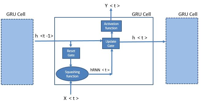
Let’s try to see this equation pictorially to get a stronger intuition of GRUs .
Note that I have not drawn the connections from Xs to the Gates for simplicity of representation. Refer to the equations for complete understanding of the mathematics behind the scene.
Here is a quick check of all you have learnt till now –
Why do you think GRU is able to mitigate the challenge of vanishing gradient?
The answer is right there in the picture. Now, we have only an update gate between h<t> and h<t-1> which has a value between 0 and 1. Our back propagation does not have to travel through the mathematically complex squashing function in a traditional RNN.
Let’s step up the game and understand Long Short Term Memory (LSTM)
LSTM is very similar to GRU but has more number of parameters to optimize. More parameters means more time to train these models. However, LSTM is supposed to perform better than GRU in sentences with long dependencies.
We will focus on key differences in mathematical formulation between LSTM and GRU, rather than trying to write the equations from scratch. This will not only build up our concept on top of our GRU understanding but also help us appreciate the key differences.
We had two gates in GRU – Update gate and the Reset Gate. LSTM does not have the Reset gate, but you are free to modify the architecture to derive your own LSTM. The Update gate in LSTM is broken down into two:
(Update) = Input                       ..........This was the first part in the GRU

(1 - Update) = Forget                  ..........This was the second part in the GRU
This is one of the key differences between LSTM and GRU, the sum of coefficient for last hidden state and new calculated RNN hidden state is constraint to sum up to 1, whereas LSTM have these two coefficients as independent variables that can take any value. Now coming to a second key difference, LSTM maintains two different memories – Cell State and Hidden state. Cell state is the long term memory and hidden state is the short term memory, very similar to human brain. The concept will get clearer once we start formulating the mathematical equation. We will denote c<t> for cell state and h<t> for the hidden state.
cRNN <t>  =  tanh(W  * (X <t>,h<t-1> )  + C)  ..............This remains same as GRU
cAlt<t> = c<t -1>                             ..............This remains same as GRU
c <t> = Input * cRNN <t> + Forget * cAlt<t>   ..............Notice that we now have Forget Gate
h<t> = Output * tanh (c <t> )                 ..............This is unique for LSTM
Input, Forget, Output = Activation(W  * (X <t>,h<t-1> )  + C)
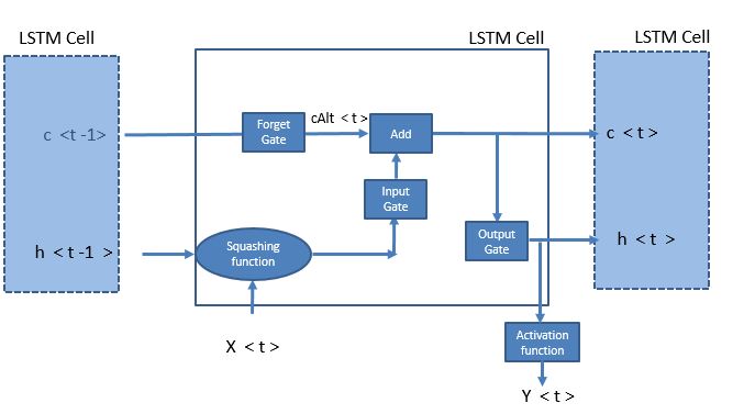
Here is a visualization of the equations written above:
Note that I have not drawn the connections from X’s to the Gates for simplicity of representation. Refer to the equations for complete understanding of the mathematics behind the scene.
Forget gate is an important difference between LSTM and GRU. This gate regulates how much previous information needs to be sent to the next cell, whereas GRU exposes its entire memory to the next cell. Note that hidden state, and not the cell state, is used to evaluate all the gates in LSTM. Hence controlling the hidden state that is moving forward to the next cell can give us complete control of all gates in the next cell. The difference is not a strong one when it comes to practical applications of LSTM vs. GRU. The cell state acts as a shortcut for the back propagation to travel and hence avoids the problem of diminishing gradient.
A short note on Bidirectional RNN
Here is a brain twister – “There ________ (seem/seems) to be a defect in all the cars manufactured by company XYZ in 2010”. What is the main subject of this sentence – “a defect” or “all the cars” or “company XYZ”? The answer might look obvious to you – “a defect” is the main subject and, hence “seems” is the right answer. Here is what I want you to think about – out of GRU and LSTM, which one is in a better position to answer this question?
Probably, none. Because both LSTM and GRU accumulate all the knowledge going from left to right. This approach works fairly well for most of the sentences, except ones that look like the example given above. In such exception cases, the relevant information that is required to answer such questions lies on the right side and is yet to be read by the algorithm. How do we solve this challenge?
Bidirectional RNN to the rescue! It works on a simple idea – just read the sentence from both left to right and right to left. This process increases our optimizing parameters space by approximately a factor of 2. Our next layer will simply have more features to work with and the rest of the architecture remains the same.
If the above explanation is too complex to grasp, just make a note in your long term memory that Bidirectional is an add-on to our LSTM and GRU cell that can simply enhance their capability to create “thought vector” from either direction at a cost of additional processing time.
LSTM vs GRU – Who wins?
There has been a lot of debate around which among the two wins without an objective answer yet. Here are a few widely accepted principles and my opinions on them:
- GRU is new and hence not as reliable as LSTM. I have personally not found this to be true, but it is true that GRU is much younger than LSTM
- GRU runs a lot faster because of the lower number of parameters. I have validated this fact and found it to be absolutely TRUE
- LSTM works better in sentences with long dependencies. I have not found this statement to be true in the limited number of problems I have worked with
- We generally start to test models using bidirectional LSTM, followed by bidirectional GRU, then LSTM, and finally GRU. If our performance does not deteriorate from moving left to right, you choose the one to the right. This is obvious as the processing time for the algorithms to the right is lesser than the ones to the left. I have found this statement to be accurate and most of the times I ended up using either bidirectional GRU or GRU.
End Notes
Even though this article included minimal mathematics, it is enough for you to start experimenting with all the architectures referenced in this article. If your end goal is to use these tools on real world problems, I will recommend further reading on sequence to sequence models (Encoder Decoder architectures). I will cover these sophisticated architectures in my future articles – stay tuned.
If you have any ideas or suggestions regarding the topic, do let me know in the comments below!


