This article was published as a part of the Data Science Blogathon.
In this post, we will discuss the sentiment analysis problem. We have taken the Twitter US airline sentiment dataset for this empirical study. We will train various classification models and compare the performance metrics to extract useful insights.
Twitter US Airline Sentiment dataset:
This dataset contains the tweets of the US airline customers, who have shared their feedback on Twitter. Tweets have been manually labeled with one of the three sentiments:- Negative, Neutral, Positive. Dataset has 14640 instances and 15 features.
# Data Loading

import pandas as pd
data = pd.read_csv('Tweets.csv')
data.dtypes
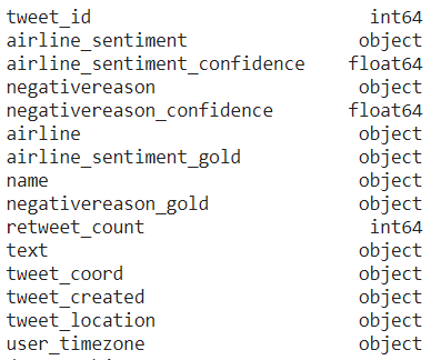
We use only the “text” and “airline_sentiment” columns for the study. Extract these columns and apply the following preprocessing steps:
1. Convert the sentiment text labels into integer labels. [Negative:0, Neutral:1, Positive:2]
2. Preprocess the input text data with TweetTokenizer (NLTK library). Replace username with wildcard. Replace numbers with wildcard. Replace emojis with the corresponding text (smiley emoji with ).
# Tweet text preprocessing...

import json
import collections
import pandas as pd
import numpy as np
from nltk.corpus import stopwords
import re
from nltk.tokenize import TweetTokenizer
def text_preprocess(text, tknzr):
    FLAGS = re.MULTILINE | re.DOTALL
    # Different regex parts for smiley faces
    eyes = r"[8:=;]"
    nose = r"['`-]?"
    # function so code less repetitive
    def re_sub(pattern, repl):
        return re.sub(pattern, repl, text, flags=FLAGS)
    text = re_sub(r"https?://S+b|www.(w+.)+S*", "")
    text = re_sub(r"/"," / ")
    text = re_sub(r"@w+", "")
    text = re_sub(r"{}{}[)dD]+|[)dD]+{}{}".format(eyes, nose, nose, eyes), "")
    text = re_sub(r"{}{}p+".format(eyes, nose), "")
    text = re_sub(r"{}{}(+|)+{}{}".format(eyes, nose, nose, eyes), "")
    text = re_sub(r"{}{}[/|l*]".format(eyes, nose), "")
    text = re_sub(r"<3","")
    text = re_sub(r"[-+]?[.d]*[d]+[:,.d]*", "")
    text = re_sub(r"([!?.]){2,}", r"1 ")
    text = re_sub(r"b(S*?)(.)2{2,}b", r"12 ")
    text = re_sub(r"[A-Za-z]+[@#$%^&*()]+[A-Za-z]*","abuse")
    tokens = tknzr.tokenize(text.lower())
    return tokens #" ".join(tokens)

tknzr=TweetTokenizer(reduce_len=True, preserve_case=False, strip_handles=False)
# Label Encoding...
from sklearn import preprocessing
le = preprocessing.LabelEncoder()
le.fit(data.airline_sentiment)
data['categorical_label'] = le.transform(data.airline_sentiment)
Now, we will discuss each model and individual performance. At last, we will compare all the models to reach the final conclusion. We have split the data into 70:30::train:test for all the models.
X = []
Y = []
for idx in data.index:
  X.append(text_preprocess(data['text'][idx], tknzr))
  Y.append(data['categorical_label'][idx])
# Train-Test splitting
from sklearn.model_selection import train_test_split
X_train, X_test, Y_train, Y_test = train_test_split(X, Y, test_size=0.3)
labels = ['Negative','Neutral', 'Positive']  # For further use...
Word-2-Vector model (Word2Vec):
Word2Vec is used to create and train semantic vector spaces consisting of several hundred dimensions based on a text corpus. In this vector space, every word of the corpus is represented as a vector. Words that share the same context are approximated closer to each other in this space. We train Word2Vec on the input training data. Next, we convert each train and test instance into a vector using the trained model (take mean of all the word vectors of an instance).
from gensim.models import Word2Vec
# train model
model = Word2Vec(X_train, min_count=1)
# Helper function
def get_w2v_vector(doc):
  tmp = []
  for w in doc:
    try:
      tmp.append(model[w])
    except:
      pass
  return np.mean(tmp, axis=0)
# Convert training text into vectors
train_vectors_w2v = []
for doc in X_train:
    try:
      train_vectors_w2v.append(get_w2v_vector(doc))
    except Exception:
      print('error...')
# Convert Test text into vectors
test_vectors_w2v = []
for doc in X_test:
    try:
      test_vectors_w2v.append(get_w2v_vector(doc))
    except Exception:
      print('error...')
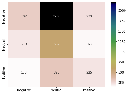
We calculate the similarity of each test vector with all the train vectors and label it with the sentiment of the most similar vector.
from sklearn.metrics.pairwise import linear_kernel
cosine_similarities = linear_kernel(train_vectors_w2v, test_vectors_w2v)
Y_pred = []
for cs in cosine_similarities.T:
    idx = cs.argsort()[-1]
    Y_pred.append(Y_train[idx])
We calculate the following metrics to evaluate the model.
from sklearn.metrics import classification_report, confusion_matrix
import seaborn as sn
import pandas as pd
import matplotlib.pyplot as plt

# This utility function will be used to evaluate the other models also.
def show_performance_data(Y_test, Y_pred, model_name):
  print(classification_report(Y_test, Y_pred, target_names=labels))
  tmp_result = classification_report(Y_test, Y_pred, target_names=labels, output_dict=True)
  cm1 = confusion_matrix(Y_test, Y_pred)
  df_cm = pd.DataFrame(cm1, index = [i for i in labels], columns = [i for i in labels])
  plt.figure(figsize = (7,5))
  sn.heatmap(df_cm, annot=True,cmap='gist_earth_r', fmt='g')
  plt.savefig('confusion_mrtx_'+model_name+'.png',bbox_inches = 'tight')
  return tmp_result

result_word2vec = show_performance_data(Y_test, Y_pred, 'word2vec')
Latent Dirichlet Allocation (LDA):
It is a topic modeling method to learn the topic representations and their distribution in a text document. We represent each document in terms of a small number of topics instead of a high-dimensional dense vector. Here, we will consider each tweet as a document and train the model. We train the LDA model on the training data with topic count 20. We represent each train and test instance in terms of 20 topics. Cosine similarity is calculated the same as Word2Vec.
import os
from gensim.corpora import Dictionary
import gensim
from gensim.matutils import cossim
topic = 20
Lda = gensim.models.ldamodel.LdaModel
dictionary = Dictionary(X_train)
train_corpus = [dictionary.doc2bow(doc) for doc in X_train]
model = Lda(corpus=train_corpus, id2word=dictionary, num_topics=topic)
test_corpus = [dictionary.doc2bow(doc) for doc in X_test]
train_x_topics, test_x_topics = [], []
# Convert text data into topic vectors
for t in train_corpus:
  train_x_topics.append(model[t])
for t in test_corpus:
  test_x_topics.append(model[t])
# Prediction
Y_pred = []
for i in range(len(test_x_topics)):
  tst = test_x_topics[i]
  sim = [cossim(tst, tr_t) for tr_t in train_x_topics]
  idx = np.array(sim).argsort()[-1]
  Y_pred.append(Y_train[idx])
Following are the results and confusion matrix for the LDA model.
result_lda = show_performance_data(Y_test, Y_pred, 'lda')


Document-2-Vector model (Doc2Vec):
Doc2Vec is an extension of the Word2Vec model. Word2Vec encodes a single word into a dense vector. Doc2Vec can encode a paragraph or document into a dense vector. The rest of the things are the same as Word2Vec. Following are the results and confusion matrix for Doc2Vec model.
from gensim.test.utils import common_texts
from gensim.models.doc2vec import Doc2Vec, TaggedDocument
vec = 100
tagged_corpus = [TaggedDocument(d, [i]) for i, d in enumerate(X_train)]
model = Doc2Vec(tagged_corpus, vector_size=vec, window=3, dm=1, min_count=1, workers=4)
Y_pred = []
for a in X_test:
  test_doc_vector = model.infer_vector(a)
  sims = model.docvecs.most_similar(positive = [test_doc_vector])
  Y_pred.append(Y_train[sims[0][0]])
result_doc2vec = show_performance_data(Y_test, Y_pred. 'doc2vec')


Universal Sentence Encoder (USE):
The USE encodes the text into n-dimensional vectors that can be used for semantic similarity, classification, clustering, and other natural language tasks. The model is trained and optimized for sentence level text, like sentences, phrases, or small paragraphs. They used versatile data sources and a variety of tasks to encompass a wide range of NLP tasks dynamically. The input is variable length English sentences, and the output is a 512-dimensional embedding. Training is not required in this case. We directly encode the train and test instances into 512-D vectors.
import tensorflow as tf
import tensorflow_hub as hub
# Loading USE encoder
module_url = "https://tfhub.dev/google/universal-sentence-encoder/4"
use_model = hub.load(module_url)
print ("module %s loaded" % module_url)
def get_use_vector(doc):
  tmp = use_model(doc)
  return np.mean(tmp, axis=0)
# Convert text data into vector
train_vectors = []
for doc in X_train:
    try:
      train_vectors.append(get_use_vector(doc))
    except Exception:
      print('error...')
test_vectors = []
for doc in X_test:
    try:
      test_vectors.append(get_use_vector(doc))
    except Exception:
      print('error...')
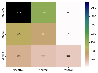
Similarity calculations are the same as Word2Vec. This model is one of the examples of Transfer learning. Following are the results of the USE model.
Y_pred = []
cosine_similarities = linear_kernel(train_vectors, test_vectors)
for cs in cosine_similarities.T:
    idx = cs.argsort()[-1]
    Y_pred.append(Y_train[idx])
result_use = show_performance_data(Y_test, Y_pred, 'use')

K Nearest Neighbor classifier (KNN):
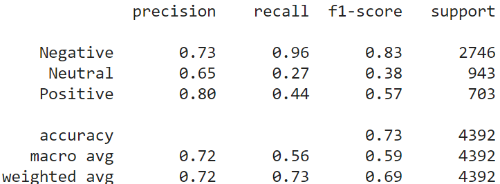
KNN is a lazy classifier. It does not perform any training on the training data. When a test instance comes, KNN calculates the distance of the test instance with all the training instances. It selects K (odd number) nearest instances and considers their labels to decide the label of the test data. We choose K=5 for the study. We have used the encoded vectors from the USE model in this part. Following are the results of the KNN model on the test data. Classification performance has increased up to 10% compared to the previous models. Still, the performance for the “Neutral” class is not at a satisfactory level.
from sklearn.neighbors import KNeighborsClassifier
neigh = KNeighborsClassifier(n_neighbors=5)
neigh.fit(train_vectors, Y_train)
Y_pred = neigh.predict(test_vectors)
result_knn = show_performance_data(Y_test, Y_pred, 'knn')

Random Forest Classifier (Ensemble Learning):
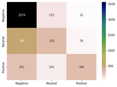
Random forest trains the N number of decision trees on the subsets of training data. This is a form of ensemble learning. Here also, we have used the USE model embeddings to represent the instances. When a test instance comes, Random Forest collectively considers the predictions of all the N decision trees to make the final prediction. The random forest has increased the performance a little bit more compared to the KNN. (N=10 in this study).
from sklearn.ensemble import RandomForestClassifier
clf = RandomForestClassifier(n_estimators=10)
clf = clf.fit(train_vectors, Y_train)
Y_pred = clf.predict(test_vectors)
result_rnmdfst = show_performance_data(Y_test, Y_pred, 'rndmfst')

Gradient Boosting Classifier (GBC):
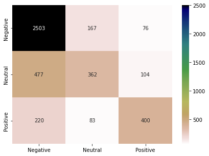
GBC is a group of multiple weak classifiers that combine them to create a single robust classifier. Generally, decision trees are used as the base units to create the final model. In this study, we have used 15 weak classifiers to build the final classification model. GBC has increased the performance by 4% compared to the random forest classifier.
from sklearn.ensemble import GradientBoostingClassifier
clf = GradientBoostingClassifier(n_estimators=15, learning_rate=1.0,max_depth=1, random_state=0).fit(train_vectors, Y_train)
Y_pred = clf.predict(test_vectors)
result_grdbst = show_performance_data(Y_test, Y_pred, 'grdbst')
Comparative Analysis:
Here, we will discuss the performance of all the models in a combined manner. Dataset has the class imbalance problem. Negative instances are present in large numbers in the dataset. Therefore, we can see all the models have achieved better precision for the “Negative” class. Surprisingly, models have performed quite well for the “Positive” class, even with the least number of instances. Word2Vec has performed worst on the test data.
N = 3
results = {'Doc2Vec':result_doc2vec, 'Word2Vec':result_word2vec, 'KNN':result_knn, 'USE':result_use, 'Random Forest':result_rnmdfst, 'Gredient Boost':result_grdbst, 'LDA':result_lda}
ind = np.arange(N)
width = 0.1
p = []
clr = ['b','g','r','c','m','k','y']
i=0
for a,b in results.items():
  tmp = [b['Negative']['precision'], b['Neutral']['precision'], b['Positive']['precision']] # replace 'precision' with 'recall' or 'f1-score' for the next two plots.
  print(tmp)
  p.append(plt.bar(ind+width*i, tmp, width, color = clr[i]))
  i+=1
plt.xlabel("Sentiments")
plt.ylabel('Precision')
plt.title("Precison comparison of all the models with respect to sentiments")
plt.xticks(ind+width,labels)
plt.legend( tuple(p), tuple(results.keys()), loc='upper center', ncol=2)
plt.show()
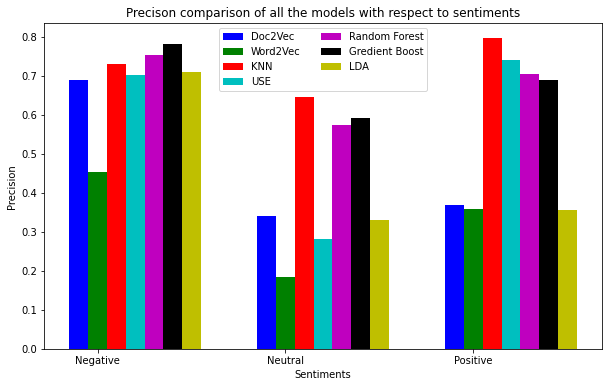
All the models have achieved a good recall score for “Negative” sentiments (except Word2Vec). In contrast to the Precision score, models have not scored a satisfactory Recall for the Positive sentiments. GBC has achieved the best Recall for the sentiments collectively.
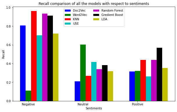
When we try to increase Recall, Precision will go down, and the visa-versa is also true. F-score captures the combined score of Recall and Precision. Thus, F-score provides the correct picture of the models’ performance. GBC, RandomForest, and KNN have performed most effectively for all three types of sentiments. The most interesting observation is on the Doc2Vec model. Doc2Vec has performed very well for the “Negative” class but failed to achieve the same performance for the other two types of sentiments.

The following bar chart represents all the models’ overall performance in terms of Precision, Recall, and F-score. Word2Vec was the least performing model among all. USE model, LDA, and Doc2Vec have shown average performance. GBC, KNN, and RandomForest have become the best model on this dataset for sentiment classification. The most important thing is that we have used USE-based embeddings to represent tweet data in KNN, GBC, and RandomForest model building.
i=0
for a,b in results.items():
  tmp = [b['weighted avg']['precision'], b['weighted avg']['recall'], b['weighted avg']['f1-score']]
  print(tmp)
  f.append(plt.bar(ind+width*i, tmp, width, color = clr[i]))
  i+=1
plt.xlabel("Metrics")
plt.ylabel('score')
plt.title("Over all weighted scores")
plt.xticks(ind+width,['Precision', 'Recall', 'F1-score'])
plt.legend( tuple(f), tuple(results.keys()), loc='upper center', ncol=7)
plt.show()

Conclusion:
In this post, we have discussed the sentiment classification problem using the US airline tweet dataset. We have discussed the results in detail to infer useful insights. Source code notebook file is available at this Collaboratory link. We can experiment with the hyperparameter to gain more information from this work. We have used only the tweet text to model the classification task. However, there are a few other columns that can be used for further exploration. Thank you.
The media shown in this article is not owned by Analytics Vidhya and are used at the Author’s discretion


