This article was published as a part of the Data Science Blogathon
Objectives
- The article focuses on building beautiful and interactive ML web apps without any web development experience!
- We will cover data loading, visualization, interaction, and generating dashboards in just a few lines of pure python code!
- The machine learning interactive dashboards will provide users to choose any classification algorithm, select evaluation metrics, and switch hyper-parameters on the go in real-time, all without any coding experience.
Introduction
Don’t you wish to build awesome interactive web applications for your machine learning projects!! but web development, not your forte?
Streamlit is your new way out! Developing and deploying powerful machine learning web apps have never been so easy!
Streamlit is an open-source python library that allows swift custom web app building revolving data science, machine learning, and much more. Streamlit aims at building and deploying applications without the necessity of any web development knowledge.
Why choose Streamlit?
Streamlit library offers a set of unique features which sets it apart.
- Pure python scripting without the need for HTML, CSS, etc.
- Data caching features available
- Fast and easy build and deployment
- Supports several data science frameworks
- Creates interactive applications without any complexity
- Offers widgets as variables
In just a few minutes we can easily generate exquisite dashboards for our machine learning project — so let’s get started!
Learning Objectives
- Use Streamlit and Python to build an interactive machine learning dashboard
- Train multiple classifiers including Logistic Regression, Random Forest, and Support Vector Classifiers
- Switch and Select hyperparameter settings for each classification algorithm
- Plot evaluation metrics for the classifiers
Setting up the application
We can set up the application in a few easy steps.
Installation
Install the python Streamlit library
pip install streamlit
Importing
Import the required libraries for the machine learning application.
from numpy.core.numeric import True_
from sklearn import metrics
import streamlit as st
import pandas as pd
import numpy as np
from sklearn.svm import SVC
from sklearn.linear_model import LogisticRegression
from sklearn.ensemble import RandomForestClassifier
from sklearn.preprocessing import LabelEncoder
from sklearn.model_selection import train_test_splitfrom sklearn.metrics import plot_confusion_matrix, plot_roc_curve, plot_precision_recall_curve
from sklearn.metrics import precision_score, recall_score
Initialization
Let’s start very simple by creating a python script that prints text to the Web application.
def main():
    st.title(“Introduction to building Streamlit WebApp”)
    st.sidebar.title(“This is the sidebar”)
    st.sidebar.markdown(“Let’s start with binary classification!!”)
if __name__ == ‘__main__’:
    main()
We can initialize the application by defining the main method. We call streamlit by st and then specify the widget or function that needs to be added to the application.
For creating the main title we use st.title. Section titles can be added by st.header or st.subheader. Streamlit also supports Markdowns by st.markdown.
We can build a sidebar for adding interactive elements so that the users can make desired choices for hyperparameter tuning and model selection
The results would be reflected on the main page. Sidebar title can be added by st.sidebar.title.
Running the application
Switch to the terminal and run the application by the following command, this should automatically open up the Web browser. And this would be running on localhost with the default port 8501- http://localhost:8501
streamlit run app.py
Any further changes made to the code in the editor will be automatically updated after saving without needing to recompile.
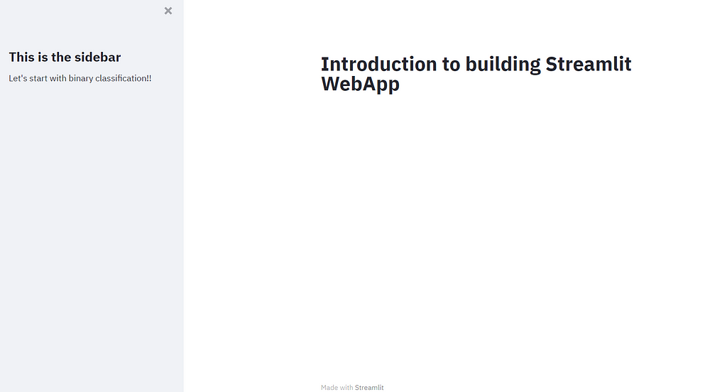
Streamlit application
Data Loading
Now we will be loading the freely available dataset from the UCI machine learning repositories, We can use this dataset for binary classification. It consists of multiple columns, and each column is of a categorical data type so we need to perform some sort of encoding to convert these categorical features into numerical data.
For the data loading process, we define a function inside the main method to read the CSV file and store it as a pandas data frame. We make a function to iterate through each column in our data frame and fit transform at the data so it’s labelled and coded.
@st.cache(persist= True)
def load():
    data= pd.read_csv("mushrooms.csv")
    label= LabelEncoder()
    for i in data.columns:
        data[i] = label.fit_transform(data[i])
return data
df = load()
And since we don’t want our app to load the data every single time any change is made to the code. For this, we can use a streamlit decorator @st.cache(persist= True) which helps us to cache the outputs to disk and use it at any time.
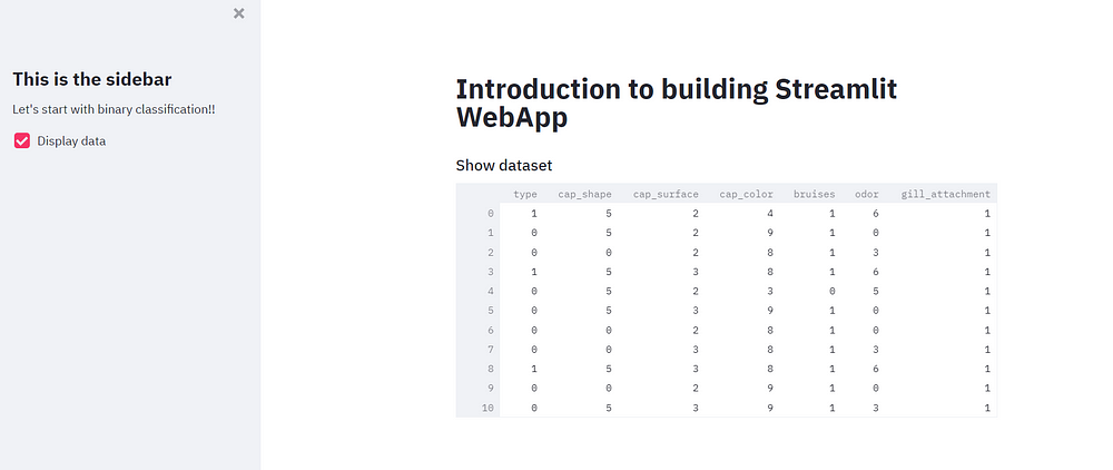
We can add the additional functionality of displaying raw data on the web app by adding a checkbox at the sidebar which would reflect the data on the main section if selected.
if st.sidebar.checkbox("Display data", False):
    st.subheader("Show Mushroom dataset")
    st.write(df)
Creating Training and Test splits
The first step for model creation is to create training and test splits. We can create a split function for the same. Now we can use the train test split function from the sklearn library to split our dataset and drop the target column.
@st.cache(persist=True)
def split(df):
    y = df.type
    x = df.drop(columns=["type"])
    x_train, x_test, y_train, y_test =     train_test_split(x,y,test_size=0.3, random_state=0)

return x_train, x_test, y_train, y_test
x_train, x_test, y_train, y_test = split(df)
Now we can move forward to model training and model evaluation.
Evaluation Metrics
We would create a function for plotting various evaluation metrics. This lets the user select any evaluation metrics such as Confusion matrix, ROC Curve and Precision-Recall Curve as it is a binary classification problem.
Create a metrics list and a subheader for creating the plots. Let us also
create a class that has two values edible and poisonous.
def plot_metrics(metrics_list):
    if "Confusion Matrix" in metrics_list:
        st.subheader("Confusion Matrix")
        plot_confusion_matrix(model, x_test, y_test, display_labels=   class_names)
        st.pyplot()
    if "ROC Curve" in metrics_list:
        st.subheader("ROC Curve")
        plot_roc_curve(model, x_test, y_test)
        st.pyplot()
    if "Precision-Recall Curve" in metrics_list:
        st.subheader("Precision-Recall Curve")
        plot_precision_recall_curve(model, x_test, y_test)
        st.pyplot()
class_names = ["edible", "poisnous"]
As soon as the selected evaluation function is called, it will create a matplotlib plot that would be displayed on the main page.
Training an SVM classifier
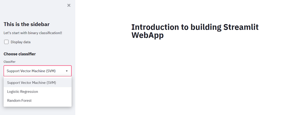
Let’s add a subheader to the sidebar allowing the user to choose a classifier. Next, we can construct a widget that shows a list of classifiers in a drop-down fashion. We can add our classifier options starting with SVM, logistic regression, and the last one as the random first question.
st.sidebar.subheader("Choose classifier")
classifier = st.sidebar.selectbox("Classifier", ("Support Vector Machine (SVM)", "Logistic Regression", "Random Forest"))
Adding SVM hyperparameters
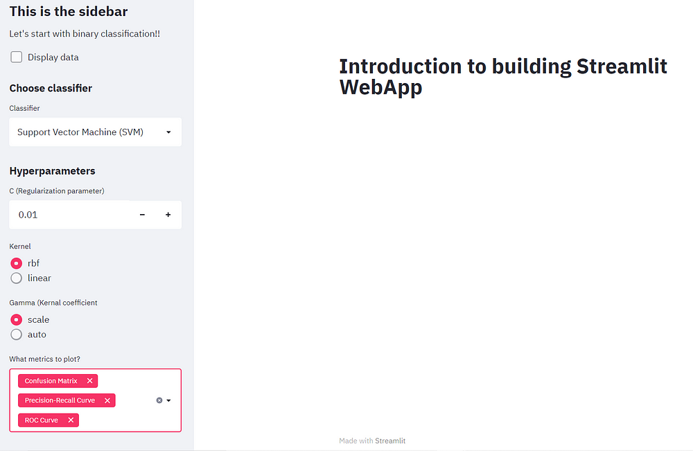
After the user selects the SVM classifier, a list of hyper-parameters is displayed. We can add a regularization parameter and provide a range of 0.1 to 10.0 which can be handled by plus and minus signs. The power of SVMs is really by choosing their kernels.
We can simply add a radio button that allows users to select from either
of two kernels — RBF and linear. And lastly, let’s add the last hyperparameter called Gamma.
As we also want the evaluation metrics to be plotted onto the web app. So let’s also add the feature that caters to the user’s required evaluation metrics for this, we can create a multi-select widget that allows the user to input one or more metrics.
if classifier == "Support Vector Machine (SVM)":
    st.sidebar.subheader("Hyperparameters")
    C = st.sidebar.number_input("C (Regularization parameter)", 0.01, 10.0, step=0.01, key="C")
    kernel = st.sidebar.radio("Kernel", ("rbf", "linear"), key="kernel")
    gamma = st.sidebar.radio("Gamma (Kernal coefficient", ("scale", "auto"), key="gamma")
metrics = st.sidebar.multiselect("What metrics to plot?", ("Confusion Matrix", "ROC Curve", "Precision-Recall Curve"))
Training Model
Moving forward towards creating the actual classifier. Firstly we shall instantiate the model and fit our training data. Followed by calculation of accuracy and then performing predictions on the test dataset.
We are not only concerned with the accuracy but also precision and recall hence we would like to display them on the main screen.
Enclose the following code in the if the block of the SVM classifier.
if st.sidebar.button("Classify", key="classify"):
    st.subheader("Support Vector Machine (SVM) results")
    model = SVC(C=C, kernel=kernel, gamma=gamma)
    model.fit(x_train, y_train)
    accuracy = model.score(x_test, y_test)
    y_pred = model.predict(x_test)
    st.write("Accuracy: ", accuracy.round(2))
    st.write("Precision: ", precision_score(y_test, y_pred, labels=class_names).round(2))
    st.write("Recall: ", recall_score(y_test, y_pred, labels=class_names).round(2))
    plot_metrics(metrics)
Awesome!! we have completed the SVM classifier allowing the user to experiment with various evaluation metric and hyperparameter tuning features
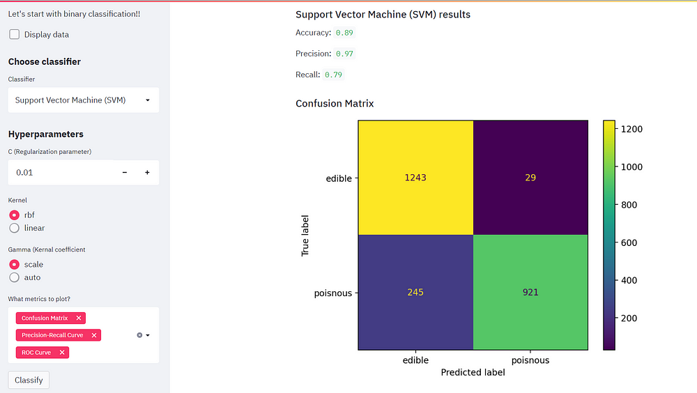
Change the regularization parameter and checkout the different evaluation metrics!
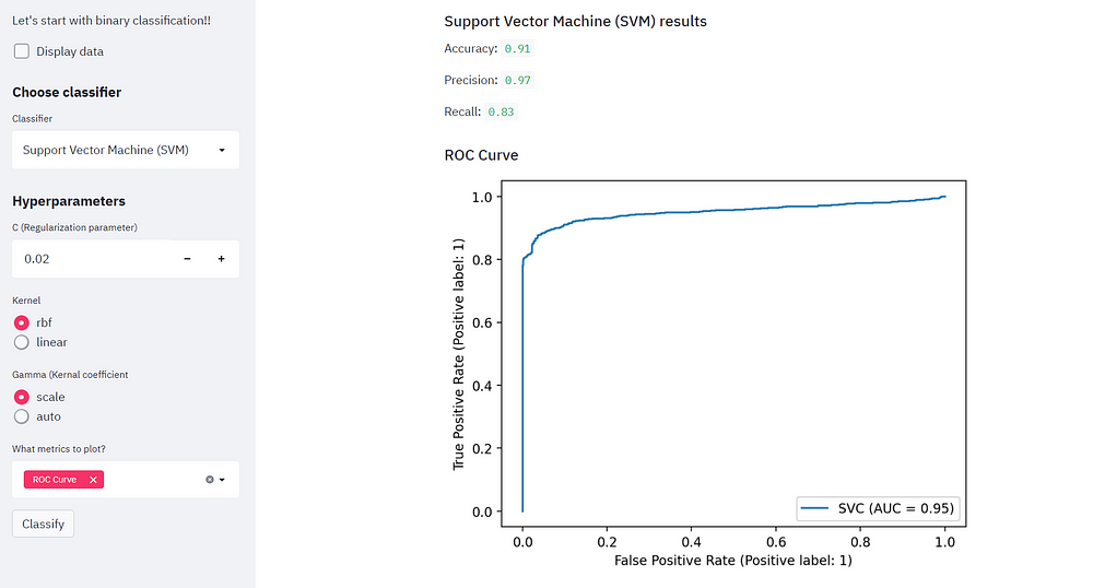
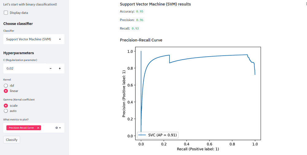
We can also switch the kernel and notice how the accuracy improves! We can analyze the same by the evaluation metrics.
Training Logistic Regression Classifier
Let’s build out the functionality for our logistic regression classifier just as we did for SVM.
Fit the logistic regression model and get the accuracy and prediction for the same and write the corresponding results on the main page. Let’s not forget to make certain minor changes such as adding a slider that will allow the user to choose the maximum iteration. Fix the lower and upper bound to 100 and 500 respectively.
Change the hyperparameters according to the logistic regression classifier and remove the Kernel and Gamma parameters.
if classifier == "Logistic Regression":
    st.sidebar.subheader("Hyperparameters")
    C = st.sidebar.number_input("C (Regularization parameter)", 0.01, 10.0, step=0.01, key="C_LR")
    max_iter = st.sidebar.slider("Maximum iterations", 100, 500, key="max_iter")
    metrics = st.sidebar.multiselect("What metrics to plot?", ("Confusion Matrix", "ROC Curve", "Precision-Recall Curve"))

    if st.sidebar.button("Classify", key="classify"):
        st.subheader("Logistic Regression Results")
        model = LogisticRegression(C=C, max_iter=max_iter)
        model.fit(x_train, y_train)
        accuracy = model.score(x_test, y_test)
        y_pred = model.predict(x_test)

        st.write("Accuracy: ", accuracy.round(2))
        st.write("Precision: ", precision_score(y_test, y_pred, labels=class_names).round(2))
        st.write("Recall: ", recall_score(y_test, y_pred, labels=class_names).round(2))
        plot_metrics(metrics)
Now we are all set for comparing the performance of both the classifiers!
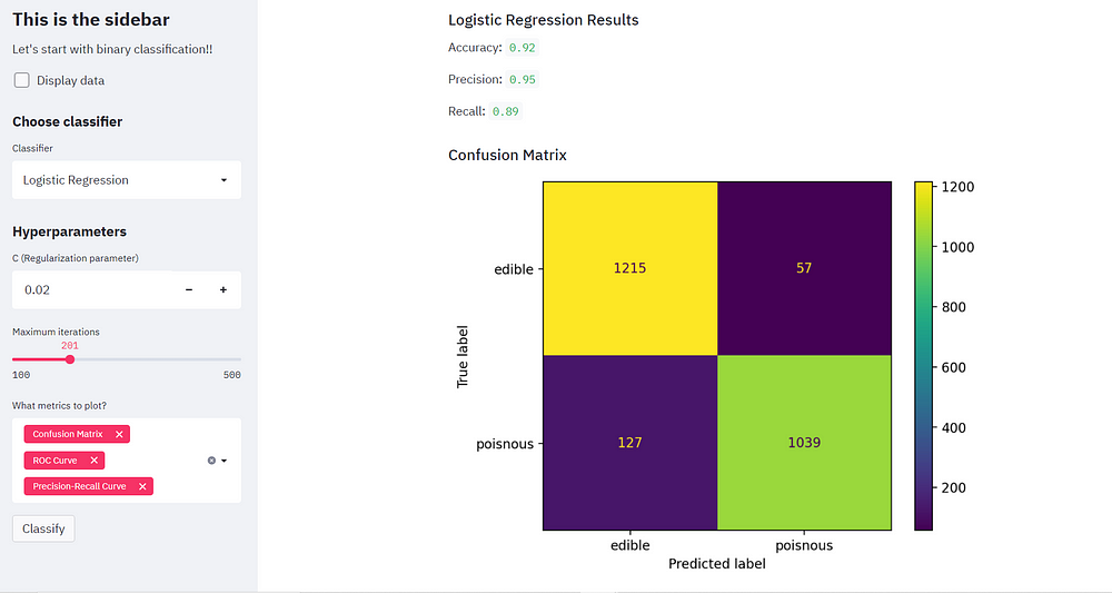
Training Random Forest classifier
Welcome to the final task of our project! Here we would create a random forest classifier. Start by clearing out the previous parameters and add new parameters such as the number of estimators that defines the number of trees in the forest for this we add an input box, set the default number as 100, and define 10 as the increment value.
Add other parameters as well, the first one being the max depth of the forest and this time set increment step by just 1. Next, we can include a radio button that allows the user to select bootstrap samples when building trees.
if classifier == "Random Forest":
    st.sidebar.subheader("Hyperparameters")
    n_estimators= st.sidebar.number_input("The number of trees in the forest", 100, 5000, step=10, key="n_estimators")
    max_depth = st.sidebar.number_input("The maximum depth of tree", 1, 20, step =1, key="max_depth")
    bootstrap = st.sidebar.radio("Bootstrap samples when building trees", ("True", "False"), key="bootstrap")

    metrics = st.sidebar.multiselect("What metrics to plot?", ("Confusion Matrix", "ROC Curve", "Precision-Recall Curve"))

    if st.sidebar.button("Classify", key="classify"):
        st.subheader("Random Forest Results")
        model = RandomForestClassifier(n_estimators=n_estimators, max_depth=max_depth, bootstrap= bootstrap, n_jobs=-1 )
        model.fit(x_train, y_train)
        accuracy = model.score(x_test, y_test)
        y_pred = model.predict(x_test)
        st.write("Accuracy: ", accuracy.round(2))
        st.write("Precision: ", precision_score(y_test, y_pred, labels=class_names).round(2))
        st.write("Recall: ", recall_score(y_test, y_pred, labels=class_names).round(2))
        plot_metrics(metrics)
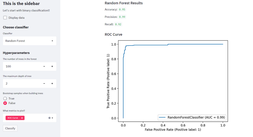
Perform classification using Random forest classifier and notice how we have very high accuracy and desirable position and recall values.
End Notes
We have successfully used the Streamlit library and Python to build a simple yet powerful machine learning WebApp.We have also learned to the title, add markdown text, and widgets such as dropdowns, radio buttons, number inputs, checkboxes, and sliders.
Not only that, we have implemented these widgets flexibly to allow the user to perform model selection and set hyperparameters, allowing users to pick various evaluation metrics.
With this hands-on project, you must have realized the real power of the streamlit library!! Streamlit allows anyone with no formal machine learning or coding background can easily work around with ML models.
The media shown in this article are not owned by Analytics Vidhya and is used at the Author’s discretion.

