This article was published as a part of the Data Science Blogathon.
Introduction
In certain circumstances, using pre-built frameworks from machine learning and deep learning libraries may be beneficial. However, you should attempt to put things into practice on your own to have good command and comprehension. This article demonstrates how to create a CNN from scratch using a custom dataset.
The most advanced method for interpreting multidimensional information, like images, is the convolutional neural network (CNN). CNN is already implemented in several packages, including TensorFlow and Keras. These libraries shield the programmer from specifics and merely provide an abstracted API to simplify life and prevent implementation complexity. However, in real life, these particulars might matter. The data analyst may occasionally need to review these particulars to boost efficiency.
In this article, we develop the CNN from scratch using a custom dataset. Convolution (Conv for short), ReLU, and max pooling are the only layers that are used in this article to form a neural network. The following are the main steps that will be covered in the article:
- Downloading the dataset from the website, then preparing the training, validation, and testing set using python3.1 and Tensorflow.
- Building own network (design the model by using Conv, Relu, and Maxpool layer)
- Train the network for 100 epochs
- Draw the training/validation accuracy and training/validation loss curve using the matplotlib library.
Importance of Deep learning for Small Data Problems
If you would work in computer vision in a formal circumstance, you’ll probably run into situations where you have to train an image classification model with relatively limited data. A “handful” of samples can be any number of photos, ranging from very few hundreds to very few hundreds of thousands. We’ll use the classification of photographs in a database of 4,000 images of cats and dogs as a working example (2,000 cats, 2,000 dogs). For training, we’ll utilize 2,000 images—1,000 for validation and 1,000 for testing.
Deep learning is frequently said to require much data to be effective. This is partially true because deep learning only works when there are many training options to suit. Deep learning might discover interesting characteristics in the training data without the requirement for handcrafted feature engineering. This is especially relevant for issues in which the input samples, like photographs, seem to be very highly complex.
However, what counts as a large number of samples varies depending on several factors, including the size and depth of the system you’re currently training. With only a few tens of observations, a Convnet cannot be trained to resolve the complex issue; however, if the job is straightforward and the framework is narrow and well regularised, a few hundred data points may be sufficient. Convnets are particularly data effective on types of tasks because they acquire local, translation-invariant features. With no need for additional feature engineering, retraining a convnet from scratch on a minimal image dataset will nevertheless produce satisfactory results despite its relative scarcity of data.
Additionally, deep-learning models are naturally very adaptable. For example, you might apply a speech-to-text or image classification model that was trained on a huge dataset for a widely differing application with only modest adjustments. In particular, several pretrained algorithms for computer vision are now freely downloadable and may be used to bootstrapping strong vision models from very little training data. These models are often trained on the ImageNet dataset. You’ll perform that in the subsequent part. Let’s start by giving you access to the information.
Downloading the CNN Dataset
The database you’ll need, Dogs vs. Cats, isn’t included with Keras. This was made public by Kaggle in 2013 as a component of a computer vision contest at a time when networks weren’t widely used. You can access the entire dataset by visiting www.kaggle.com/c/dogs-vs-cats/data.
The 543 MB dataset has 25,000 photos of dogs and cats, 12,500 of each class (compressed). After downloading and unzipping it, you’ll generate a new database with 3 groups: a training set with 1,000 samples of each class, a validation set with 500 samples of each class, and a test set with 500 samples of each class.
The code for generating the new dataset is as follows:
import os, shutil
original_dataset_dir = '/content/drive/MyDrive/Colab/Dataset/kaggle_original_data/Train/train'
base_dir = '/content/drive/MyDrive/Colab/Dataset/kaggle_original_data/cats_and_dogs_small'
os.mkdir(base_dir)
train_dir = os.path.join(base_dir, 'train')
os.mkdir(train_dir)
validation_dir = os.path.join(base_dir, 'validation')
os.mkdir(validation_dir)
test_dir = os.path.join(base_dir, 'test')
os.mkdir(test_dir)
train_cats_dir = os.path.join(train_dir, 'cats')
os.mkdir(train_cats_dir)
train_dogs_dir = os.path.join(train_dir, 'dogs')
os.mkdir(train_dogs_dir)
validation_cats_dir = os.path.join(validation_dir, 'cats')
os.mkdir(validation_cats_dir)
validation_dogs_dir = os.path.join(validation_dir, 'dogs')
os.mkdir(validation_dogs_dir)
test_cats_dir = os.path.join(test_dir, 'cats')
os.mkdir(test_cats_dir)
test_dogs_dir = os.path.join(test_dir, 'dogs')
os.mkdir(test_dogs_dir)
fnames = ['cat.{}.jpg'.format(i) for i in range(1000)]
for fname in fnames:
  src = os.path.join(original_dataset_dir, fname)
  dst = os.path.join(train_cats_dir, fname)
  shutil.copyfile(src, dst)
fnames = ['cat.{}.jpg'.format(i) for i in range(1000, 1500)]
for fname in fnames:
  src = os.path.join(original_dataset_dir, fname)
  dst = os.path.join(validation_cats_dir, fname)
  shutil.copyfile(src, dst)
fnames = ['cat.{}.jpg'.format(i) for i in range(1500, 2000)]
for fname in fnames:
  src = os.path.join(original_dataset_dir, fname)
  dst = os.path.join(test_cats_dir, fname)
  shutil.copyfile(src, dst)
fnames = ['dog.{}.jpg'.format(i) for i in range(1000)]
for fname in fnames:
  src = os.path.join(original_dataset_dir, fname)
  dst = os.path.join(train_dogs_dir, fname)
  shutil.copyfile(src, dst)
fnames = ['dog.{}.jpg'.format(i) for i in range(1000, 1500)]
for fname in fnames:
  src = os.path.join(original_dataset_dir, fname)
  dst = os.path.join(validation_dogs_dir, fname)
  shutil.copyfile(src, dst)
fnames = ['dog.{}.jpg'.format(i) for i in range(1500, 2000)]
for fname in fnames:
  src = os.path.join(original_dataset_dir, fname)
  dst = os.path.join(test_dogs_dir, fname)
  shutil.copyfile(src, dst)
print('total training cat images:', len(os.listdir(train_cats_dir)))
print('total training dog images:', len(os.listdir(train_dogs_dir)))
print('total validation cat images:', len(os.listdir(validation_cats_dir)))
print('total validation dog images:', len(os.listdir(validation_dogs_dir)))
print('total test cat images:', len(os.listdir(test_cats_dir)))
print('total test dog images:', len(os.listdir(test_dogs_dir)))
##--The total training images are--##
total training cat images: 1000
total training dog images: 1000
total validation cat images: 500
total validation dog images: 500
total test cat images: 500
total test dog images: 500
The 2,000 training images, 1,000 validation images, and 1,000 test images are all present in the respective directories. This is a binary classification problem. Therefore, classification accuracy will be a suitable metric of success. Each split comprises the same number of observations out of each class.
Building your Own CNN
You ought to be comfortable with compact Convnets. The CNN is a stacking of alternating Conv2D (with Relu as an activation function) and MaxPooling2D layers, and you’ll utilize the same overall structure.
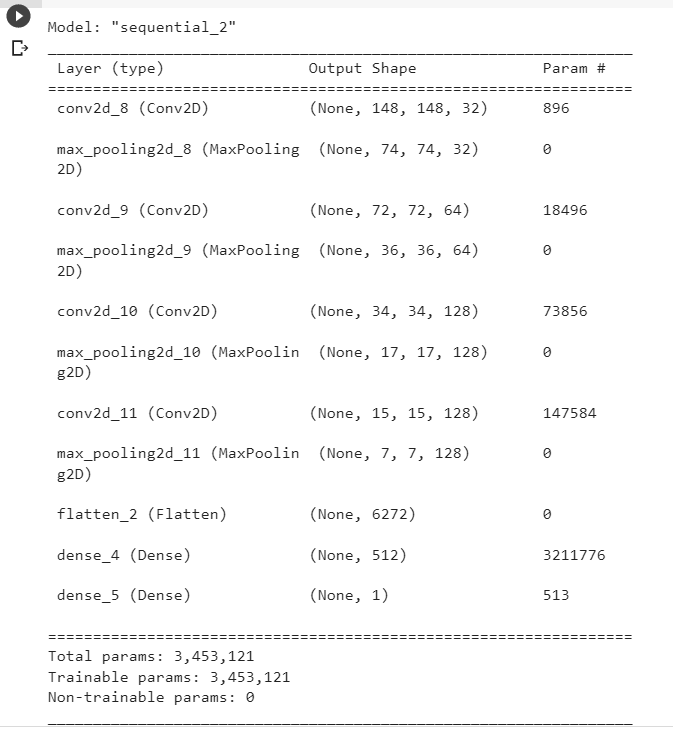
However, because you are working with larger images and a more challenging problem, you will need to expand your networks and add the Conv2D + MaxPooling2D stage. This increases the network’s capability and further reduces the dimension of the feature maps so that they aren’t too big when you get to the Flatten layer. Here, you start with the input of size 150 x 150, and immediately before the Flatten layer, you end up with feature maps of size 7 x 7.
You’ll terminate the network with a single unit (a Dense layer of size 1) and a sigmoid activation since you’re tackling a binary-classification task. This unit will encode the likelihood that the network focuses on one class over another.
Instantiating a Small CNN for Dogs vs. Cats Classification
###-----Build Your Model------###
from keras import layers

from keras import models

model = models.Sequential()

model.add(layers.Conv2D(32, (3, 3), activation='relu',input_shape=(150, 150, 3)))

model.add(layers.MaxPooling2D((2, 2)))

model.add(layers.Conv2D(64, (3, 3), activation='relu'))

model.add(layers.MaxPooling2D((2, 2)))

model.add(layers.Conv2D(128, (3, 3), activation='relu'))

model.add(layers.MaxPooling2D((2, 2)))

model.add(layers.Conv2D(128, (3, 3), activation='relu'))

model.add(layers.MaxPooling2D((2, 2)))

model.add(layers.Flatten())

model.add(layers.Dense(512, activation='relu'))

model.add(layers.Dense(1, activation='sigmoid'))
model.summary()

You’ll use the RMSprop optimizer during the compilation stage, as normal. You will use binary cross entropy as the loss so because networks ended with a single sigmoid unit.
Configuring the model for training:
####----Configuring the model for training-----####
from tensorflow import keras
from keras import optimizers
model.compile(loss='binary_crossentropy', optimizer=keras.optimizers.RMSprop(lr=1e-4), metrics=['acc'])
Data preprocessing:
#####-----Data Preprocessing-----######

from keras.preprocessing.image import ImageDataGenerator

train_datagen = ImageDataGenerator(rescale=1./255)

test_datagen = ImageDataGenerator(rescale=1./255)

train_generator = train_datagen.flow_from_directory(train_dir, target_size=(150, 150), batch_size=20, class_mode='binary')

validation_generator = test_datagen.flow_from_directory(validation_dir, target_size=(150, 150), batch_size=20, class_mode='binary')

for data_batch, labels_batch in train_generator:

print('data batch shape:', data_batch.shape)

print('labels batch shape:', labels_batch.shape)

break
Found 2000 images belonging to 2 classes.

Found 1000 images belonging to 2 classes.

data batch shape: (20, 150, 150, 3)

labels batch shape: (20,)
Let’s use the generator to fit the model to the data. You achieve this by using the fit_generator function, which is the equivalent of fit for data generators like this one. It anticipates a Python generator that, like this one, may produce batches of inputs and outputs forever as its first parameter. The Keras model wants to know how many observations to take from the generator before calling an epoch because data is created indefinitely. The steps_per_epoch option serves this purpose: the fitting process will move on to the following epoch after pulling steps per epoch batches from the generator or running for steps per epoch gradient descent steps. Since there are 20 samples in each batch, it will take 100 batches to get your target 2000 results.
Like the fit function, you can give a validation data parameter using fit_generator. It’s crucial to remember that this parameter might be either a data generator or a tuple of Numpy arrays. You must also provide the validation_steps parameter, which instructs the algorithm on how many batches to take from the validation-generator for evaluation. If you provide a generator as validation data, it is understood that this generator will output batches of validation data indefinitely.
####----Fit the Model----####
history = model.fit_generator(train_generator, steps_per_epoch=100, epochs=30, validation_data=validation_generator, validation_steps=50)
######-----Save the Model-------######
model.save('cats_and_dogs_small_1.h5')
Displaying Curves of Loss and Accuracy During Training
######-----Displaying curves of loss and accuracy during training-------######
import matplotlib.pyplot as plt
acc = history.history['acc']
val_acc = history.history['val_acc']
loss = history.history['loss']
val_loss = history.history['val_loss']
epochs = range(1, len(acc) + 1)
plt.plot(epochs, acc, 'r', label='Training acc')
plt.plot(epochs, val_acc, 'b', label='Validation acc')
plt.title('Training and validation accuracy')
plt.legend()
plt.figure()
plt.plot(epochs, loss, 'r', label='Training loss')
plt.plot(epochs, val_loss, 'b', label='Validation loss')
plt.title('Training and validation loss')
plt.legend()
plt.show()


Conclusion
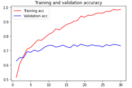
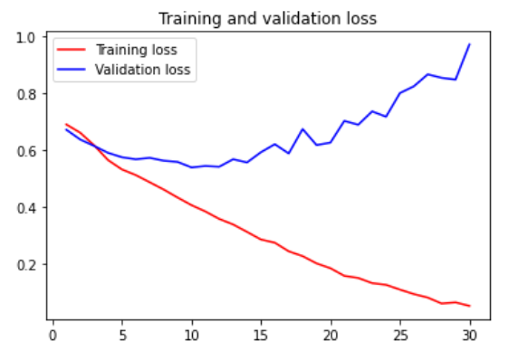
This article provides a detailed analysis of training a CNN from scratch. A custom dataset is designed by using Kaggle (cat and dog) dataset, which is available online. We have designed our CNN with our custom layer and trained it over 100 epochs. The model summary, along with the trainable and non-trainable parameters, is also discussed. After training over 100 epochs, the training and validation accuracy has been plotted. Also, the training loss and validation loss is also plotted in the figure. After analyzing the curve, we can say that:
- Plots like these characterize overfitting. While the validation accuracy plateaus around 70–72 %, the training accuracy rises linearly with time to reach over 100%.
- The training loss decreases linearly until it almost reaches zero, while the validation loss hits its lowest only after 5 epochs and then stops.
- Overfitting will be the main worry since you only have 2,000 training data. You are already aware of some methods that can lessen over fittings, such as dropout and weight decay (L2 regularization).
- In the next article, we’ll deal with a brand-new one, data augmentation, which is unique to computer vision and utilized everywhere when deep-learning models are employed to interpret images.
The media shown in this article is not owned by Analytics Vidhya and is used at the Author’s discretion.


