


Sports are filled with emotions! Cheering of audience, reactions to events on various media channels are some of the factors, which make a huge impact on the mind of the players.
![]()
If people support you, your chances to win are greatly enhanced. Live example of this fact, are the statistics of Indian cricket team playing in India and abroad. The win rate of Indian cricket team in India is approximately twice the win rate abroad.
Football is again a game driven largely by emotions. Cards (Yellow/Red), have been kept in the game to limit these emotions. If you think about places, where people express their emotions, Facebook and Twitter come out on top of the list. In this article we will make a prediction using a simplistic algorithm on the winner of 2014 FIFA world cup. This prediction will be based on the emotions expressed by people on Twitter. The entire code has been shared on github. We will just keep bits and pieces of this code as a reference in this article.
[stextbox id=”section”] Fetching the tweets on the 4 shortlisted teams [/stextbox]
The first step is to fetch the tweets, which have a reference to both FIFA and a team (out of 4). We have done this using hashtags on twitter. In this case we have put an upper threshold of 1000 tweets because of constrained hardware resources. You can use the following code to fetch the same :
[stextbox id=”grey”]
ARG.list <- searchTwitter(‘#ARG #FIFA’, n=1000, cainfo=”cacert.pem”)
ARG.df = twListToDF(ARG.list)
BRA.list <- searchTwitter('#BRA #FIFA', n=1000, cainfo="cacert.pem")
BRA.df = twListToDF(BRA.list)
GER.list <- searchTwitter('#GER #FIFA', n=1000, cainfo="cacert.pem")
GER.df = twListToDF(GER.list)
NED.list <- searchTwitter('#NED #FIFA', n=1000, cainfo="cacert.pem")
NED.df = twListToDF(NED.list)
[/stextbox]
[stextbox id=”section”] Sentiment analysis [/stextbox]
Once we have all the tweets, we need to clean the tweets and then check the sentiment of these tweets. Following is the code, I have used to pull out cleaned words and map them to a positive and negative strings.
[stextbox id=”grey”]
score.sentiment = function(sentences, pos.words, neg.words,.progress=’none’)
{
require(plyr)
require(stringr)
scores = laply(sentences, function(sentence, pos.words, neg.words) {
# clean up sentences with R's regex-driven global substitute, gsub():
sentence = gsub(":)", 'awsum', sentence)
sentence = gsub('[[:punct:]]', '', sentence)
sentence = gsub('[[:cntrl:]]', '', sentence)
sentence = gsub('\\d+', '', sentence)
# and convert to lower case:
sentence = tolower(sentence)
# split into words. str_split is in the stringr package
word.list = str_split(sentence, '\\s+')
# sometimes a list() is one level of hierarchy too much
words = unlist(word.list)
# compare our words to the dictionaries of positive & negative terms
pos.matches = match(words, pos.words)
neg.matches = match(words, neg.words)
# match() returns the position of the matched term or NA
# we just want a TRUE/FALSE:
pos.matches = !is.na(pos.matches)
neg.matches = !is.na(neg.matches)
# and conveniently enough, TRUE/FALSE will be treated as 1/0 by sum():
score = sum(pos.matches) - sum(neg.matches)
return(score)
}, pos.words, neg.words, .progress=.progress )
scores.df = data.frame(score=scores, text=sentences)
return(scores.df)
}
#Load sentiment word lists
hu.liu.pos = scan('C:/temp/positive-words.txt', what='character', comment.char=';')
hu.liu.neg = scan('C:/temp/negative-words.txt', what='character', comment.char=';')
#Add words to list
pos.words = c(hu.liu.pos, 'upgrade', 'awsum')
neg.words = c(hu.liu.neg, 'wtf', 'wait','waiting', 'epicfail', 'mechanical',"suspension","no")
[/stextbox]
[stextbox id=”section”] Scoring each tweet [/stextbox]
Once we have a well defined function which can score the tweets individually, we now score out tweets after converting them to factors (Refer to the github code).
[stextbox id=”grey”]
ARG.scores = score.sentiment(ARG.df$text, pos.words,neg.words, .progress=’text’)
BRA.scores = score.sentiment(BRA.df$text, pos.words,neg.words, .progress=’text’)
NED.scores = score.sentiment(NED.df$text,pos.words,neg.words, .progress='text')
GER.scores = score.sentiment(GER.df$text,pos.words,neg.words, .progress='text')
ARG.scores$Team = 'Argentina'
BRA.scores$Team = 'Brazil'
NED.scores$Team = 'Netherland'
GER.scores$Team = 'Germany'
head(all.scores)
all.scores = rbind(ARG.scores, NED.scores, GER.scores,BRA.scores)
[/stextbox]
[stextbox id=”section”] Summarizing the processed score [/stextbox]
Once we have a sentiment score against each tweet, we now try to summarize the score and fetch useful information from the same. You can use the following code to do the summarization
[stextbox id=”grey”]
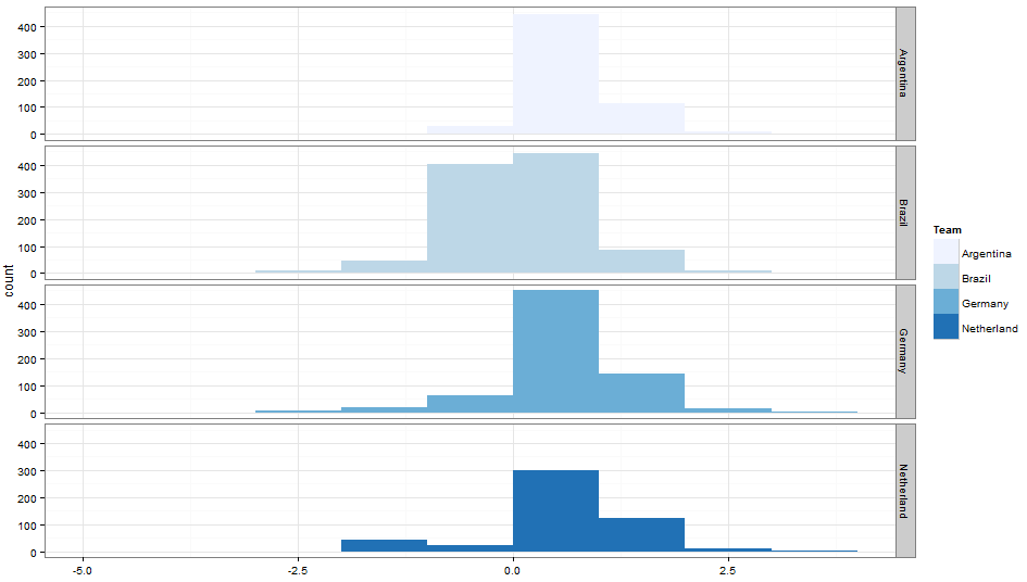
table(all.scores$score,all.scores$Team)
ggplot(data=all.scores) + # ggplot works on data.frames, always geom_bar(mapping=aes(x=score, fill=Team), binwidth=1) + facet_grid(Team~.) + # make a separate plot for each hashtag theme_bw() + scale_fill_brewer() # plain display, nicer colors
[/stextbox]
[stextbox id=”section”] Final Results [/stextbox]
As you can clearly see, we have a clear winner from the graphs i.e. Argentina. Let’s summarize this dataset into a cross tab.
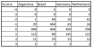
#Tweets with a +ve/-ve score for each team
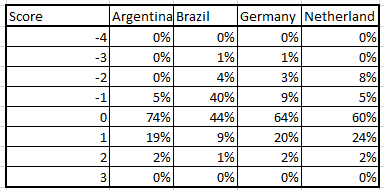
%Tweets with a +ve/-ve score for each team
Final Summary
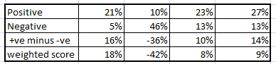
We can use different parameters to come up with the rank ordering. I have considered following to rank order teams :
Criterion 1 : %positive tweet – %negative tweets
Criterion 2 : weighted score
Criterion 3 : Fixture of matches
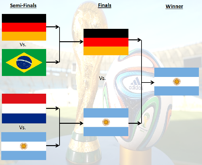
Using all three, we see our clear winner is Argentina and Brazil is clearly on rank 4. But Germany and Netherland are really close. But using the 3rd criterion, we see Germany is the one competing against Brazil. Hence, we have a clear rank order. The prediction can be seen in the 1st picture of the article.
[stextbox id=”section”] End Notes [/stextbox]
I am not a follower of the sport: football, but this analysis has excited me enough to compare my prediction to the actuals. I see myself as an unbiased analyst to make this prediction. The technique used in this article, is an over simplistic model to make such a strong prediction, but a good point to start one.
An actual model should have all kinds of input like past performance of each team versus each other, venue, players injured and finally the sentiment feed. I will like to hear more inputs to make this model more accurate. These recommendation can be used to either enhance the sentiment analysis algorithm or to include new types of input variables. People who follow the sport will be the best ones to make recommendations on this.
Here is another application – if you feel strongly against this prediction, or have your own algorithm to predict a winner – you can use the difference in the two models to create a nice betting strategy!
Did you find the article useful? Have you worked on similar objective before? How can we enhance this code to make more accurate predictions? Share with us similar kinds of post to enable us make a even stronger model.
If you like what you just read & want to continue your analytics learning, subscribe to our emails, follow us on twitter or like our facebook page.
Tavish Srivastava, co-founder and Chief Strategy Officer of Analytics Vidhya, is an IIT Madras graduate and a passionate data-science professional with 8+ years of diverse experience in markets including the US, India and Singapore, domains including Digital Acquisitions, Customer Servicing and Customer Management, and industry including Retail Banking, Credit Cards and Insurance. He is fascinated by the idea of artificial intelligence inspired by human intelligence and enjoys every discussion, theory or even movie related to this idea.