This article was published as a part of the Data Science Blogathon
Introduction
Feature engineering sounds so complicated but Nah! it’s really not. So what is feature engineering?
For me, it’s moulding data features (columns) according to one’s needs. Example: Carron told me that he bought 10 hotdogs at 20 bucks each( i.e. 20 bucks for 1 hotdog). But what I really want is a total prize of 10 hotdogs. So I created total price =200 bucks(10 times 20) in my mind. This total price works for me and this is exactly what feature engineering is. I turned the given data into something that makes more sense to me and my needs by adding new features to it.
Feature Engineering: A field of data science that creates new features or update given features of a given dataset or datasets such that it suits our and our team’s purpose is called feature engineering. It makes data more informatively readable
Now you can’t do everything in mind so we use tools like Excel, SQL, Python, R, and whatnot, by the way, you can also use pen and paper.
Let’s go R!
R is a programming language for data science work( mostly used that way). You can use R for everything from adding 1+2 to creating heavy data science algorithms.
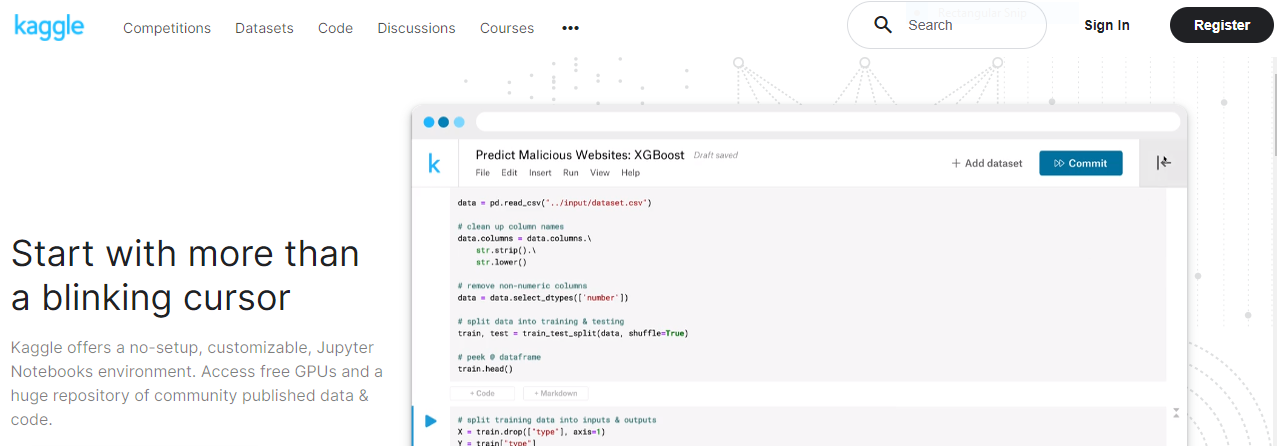
If you are new to R, no worries I got you. Just have a basic overview of R. First we need an IDE (Integrated development environment) to work with it. R studio is a good choice for your PC. But I will recommend you to use the kaggle website’s notebook. Why? because it’s kaggle( A website with lots of datasets, a dedicated working environment for you, tutorials, competitions and more).
Here https://www.kaggle.com/.
Now let’s get our hands dirty:

Go ahead and Register
- After signing in create your profile by adding images and doing essentials.
- For this tutorial, you will only download one dataset(cycling data for the first 3 months of
2019): - Direct Link or Indirect link and choose file Divvy_Trips_2019_Q1.zip then extract it.
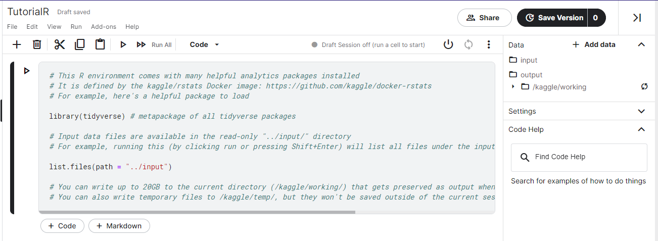
- Add this data to your kaggle notebook. For that go to the code section from the menu and click new notebook. Then you will see add data at the top right in your notebook and then upload the downloaded dataset.
- After that switch from python to R from code dropdown.

Dataset
This dataset is from a cycle company that organizes events, each having some time duration. We need to understand why customers are not becoming subscribers.
Let’s see and understand our data:
# first we will read our csv(comma separated values) using read.csv(path)
# kaggle_path is the path in kaggle where you uploaded your dataset
# note do not enter my data link add yours like kaggle_path <- " file link "
kaggle_path <- "../input/cycle-data/Divvy_Trips_2019_Q1.csv"
raw_data <- read.csv(Kaggle_path)
# lets see our data using head(raw_data) or understand using str()
str(raw_data) # or glimpse(raw_data) glimpse is from dplyr package # it give nice view

Problems:
- Just by looking at data we can tell start_time and end_time are not given as date (represented as chr) but they are real dates and time.
- And the trip duration is an integer type of data but it is shown as a character.
Converting start_time and end_time into the timestamp
as.Date(column_name): This function allows you to change into date example:
“09-09-12” will be converted to a date: 09-09-12. But what is the difference between chr and dates? The difference is date format is R’s way to store data, so “09-09-12” is not a date for R they are just characters but as.Date(c(“09-09-12”)) is a date format for R. [Note: it counts date from 01 Jan 1970.]
as.Date() does not work with time, it won’t understand time. Example as.Date(c(“09-09-12 00:10:29”)) gives 09-09-12 only and ignores 00:10:29.
as.POSIXlt(column_name)/as.POSIXct(column_name): These two functions help you to convert date and time, making a complete time stamp. Now if you will type as.POSIXlt(“09-09-12 00:10:29”)/as.POSIXct(“09-09-12 00:10:29”) you will get 09-09-12 00:10:29 as a time stamp object. Beware these function are different in a way that one stores data in list and other count it from 01 Jan 1970.
Let’s see an example:
# Converting start_time as date-time

# $ is used to specify a column of raw_data i.e. start_time

# notice how I am reassigning the converted columns to the data columns using <-

tester <- raw_data$start_time # for demonstrating as.Date()

tester<- as.Date(tester)

raw_data$start_time<-as.POSIXlt(raw_data$start_time) # for start time

raw_data$end_time<-as.POSIXlt(raw_data$end_time) # for end time

print("as.POSIXlt()")

str(raw_data$start_time)

print("as.Date()")

str(tester) # as.data.frame is used to convert into dataframe

Output

[1] "as.POSIXlt()"
POSIXlt[1:365069], format: "2019-01-01 00:04:37" "2019-01-01 00:08:13" "2019-01-01 00:13:23" ...
[1] "as.Date()"
Date[1:365069], format: "2019-01-01" "2019-01-01" "2019-01-01" "2019-01-01" "2019-01-01" ...

Now lets check our data's structure using str(raw_data)

Output:


'data.frame': 365069 obs. of 12 variables:
$ trip_id : int 21742443 21742444 21742445 21742446 21742447 21742448 21742449
$ start_time : POSIXlt, format: "2019-01-01 00:04:37" "2019-01-01 00:08:13" ...
$ end_time : POSIXlt, format: "2019-01-01 00:11:07" "2019-01-01 00:15:34" ...
$ bikeid : int 2167 4386 1524 252 1170 2437 2708 2796 6205 3939 ...
$ tripduration : chr "390.0" "441.0" "829.0" "1,783.0" ...
.... and so on
Converting character into integer and dealing with N/A
as.integer(value): This function is used to convert the value into integer data type so that we can do calculations. Let’s see our code.
raw_data$tripduration <- as.integer(raw_data$tripduration) # we'll get a surprise here
str(raw_data$tripduration)

Did you get a surprise warning? yeah, that was my intention. So what does it? It means that your code will work but there are na(N/A) values there. N/A’s are those values that mean nothing to us and R so we need to take care of them.
Look there are various ways to deal with them like replacing them with some suitable value ( something that makes sense and does not spoil or play with our data). Doing that is easy but it’s not about the method but it’s about your knowledge + intuition + experience. I will show you only one way here. Perhaps, I will create a separate blog for imputing values.
Now if you’ll see tripduration, it means time taken during a trip. If you’ll see our data ( str(raw_data) ) then you will see two columns start_time and end_time. If we will subtract the trip’s end time and the trip’s start time (end_time-start_time) you should get trip duration. So let’s check if we have the same trip durations, if yes then we will replace our tripduration with end_time-start_time.
tester <- 60*(raw_data$end_time - raw_data$start_time) # 60 is multiplied to convert min into sec
Ignore output line: time difference in mins as we explicitly converted it into seconds.

Woohoo! A perfect match…
Next, assign a tester to our tripduration replacing old values.
raw_data$tripduration <- tester
Power of Data and Time
Now we can use our start_time (type: POSIXlt date) and figure out weekdays (“Monday”, “Tuesday”… and so on ), week_number (number of weeks from 1 Jan) and month_number for month number. This is important when you need January data or weekly grouped data.
install.packages("lubridate")
library(lubridate)
raw_data$weekdays <-weekdays(raw_data$start_time) # Creates new column weekdays
raw_data$week_number <-lubridate::week(raw_data$start_time) # using lubridate's week function (::)
raw_data$month_number <-month(raw_data$start_time)
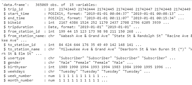
str(raw_data)
Output:

Beautiful! you made it. Great job, we learnt about how to create columns, update them, clean them and convert them. Using this basic stuff you will surely do something remarkable. All the best !!!
Hints and Tips: During the analysis and feature engineering we also use summary or describe function to view stats of our data. Like:
install.packages("psych")
library(psych) # use psych to use describe function
describe(dataset_dataframe) # first install psych
summary(dataset_dataframe)
Conclusion and what’s next!
This is just basics but our data looks a lot cleaner and more useful. An analyst will definitely like it. Now I want you to correct one thing in the data which is the birth year column. Observe it, it will have a lot of N/A values think of replacing them. (Hint: using mean, median, mode or whatever your data!).
My kaggle notebook link: click here.
The media shown in this article are not owned by Analytics Vidhya and are used at the Author’s discretion.


