Steps to Complete a Machine Learning Project

Introduction

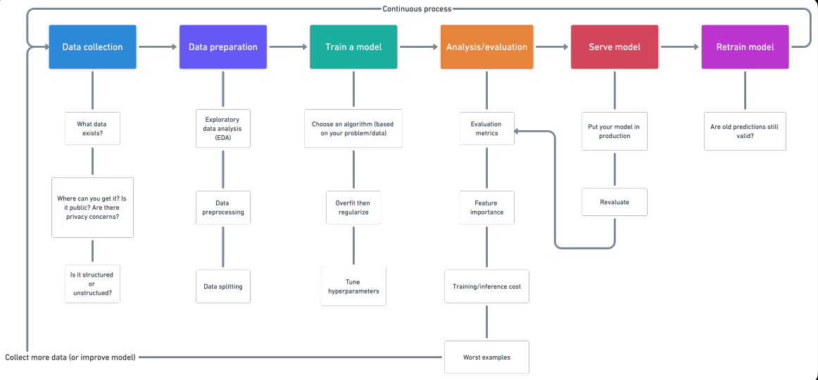
This article describes various steps involved in a machine learning project. There are standard steps that you’ve to follow for a data science project. For any project, first, we have to collect the data according to our business needs. The next step is to clean the data like removing values, removing outliers, handling imbalanced datasets, changing categorical variables to numerical values, etc.

After that training of a model, use various machine learning and deep learning algorithms. Next, is model evaluation using different metrics like recall, f1 score, accuracy, etc. Finally, model deployment on the cloud and retrain a model. So let’s start:

1. Data Collection

• Questions to ask? 

1. What kind of problem are we trying to solve?
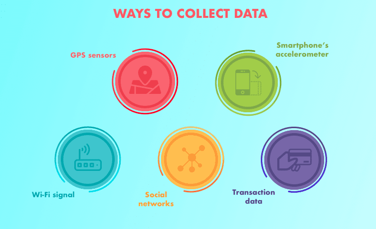
2. What data sources already exist?
3. What privacy concerns are there?
4.  Is the data public?
5.  Where should we store the files?

• Types of data

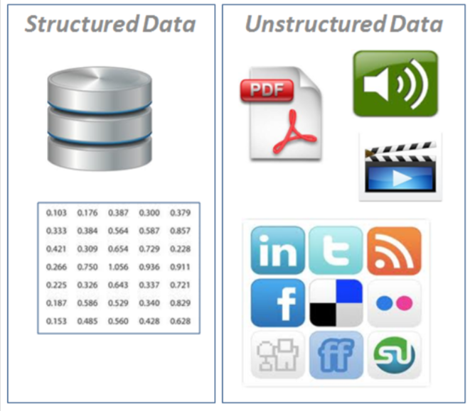
1. Structured data: appears in tabulated format (rows and columns style, like what you’d find in an Excel spreadsheet). It contains different types of data, for example numerical, categorical, time series.

• ·Nominal/categorical – One thing or another (mutually exclusive). For example, for car scales, color is a category. A car may be blue but not white. An order does not matter.

• Numerical: Any continuous value where the difference between them matters. For example, when selling houses, $107,850 is more than $56,400.

• Ordinal: Data which has order but the distance between values is unknown. For example, a question such as, how would you rate your health from 1-5? 1 being poor, 5 being healthy. You can answer 1,2,3,4,5 but the distance between each value doesn’t necessarily mean an answer of 5 is five times as good as an answer of 1.Time-series: Data across time. For example, the historical sale values of Bulldozers from 2012-2018.

• Time-series: Data across time. For example, the historical sale values of Bulldozers from 2012-2018.

1. Unstructured data: Data with no rigid structure(images, video, speech, natural
   language text)

2. Data preparation

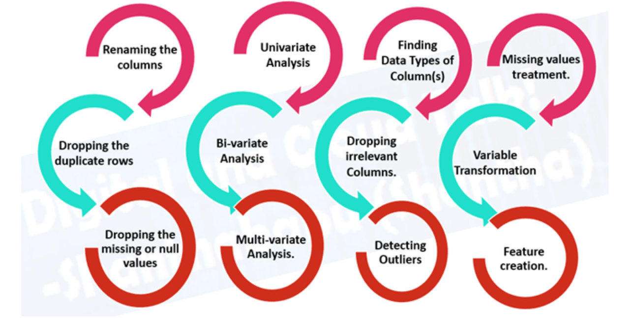
•  Exploratory data analysis(EDA), learning about the data you’re working with 

1. What are the feature variables (input) and the target variable (output) For example, for predicting heart disease, the feature variables may be a person’s age, weight, average heart rate, and level of physical activity. And the target variable will be whether or not they have a disease
2.  What kind of do you have? Structured, unstructured, numerical, time series. Are there missing values? Should you remove them or fill them feature imputation.
3.  Where are the outliers? How many of them are there? Why are they there?  Are there any questions you could ask a domain expert about the data? For example, would a heart disease physician be able to shed some light on your heart disease dataset?

• Data preprocessing, preparing your data to be modelled.

•  Feature imputation: filling missing values ( a machine learning model can’t learn
  on data that’s isn’t there)

1. Single imputation: Fill with mean, a median of the column.
2. Multiple imputations: Model other missing values and with what your model finds.
3. KNN (k-nearest neighbors): Fill data with a value from another example that is similar.
4. Many more, such as random imputation, last observation carried forward (for time series), moving window, and most frequent.

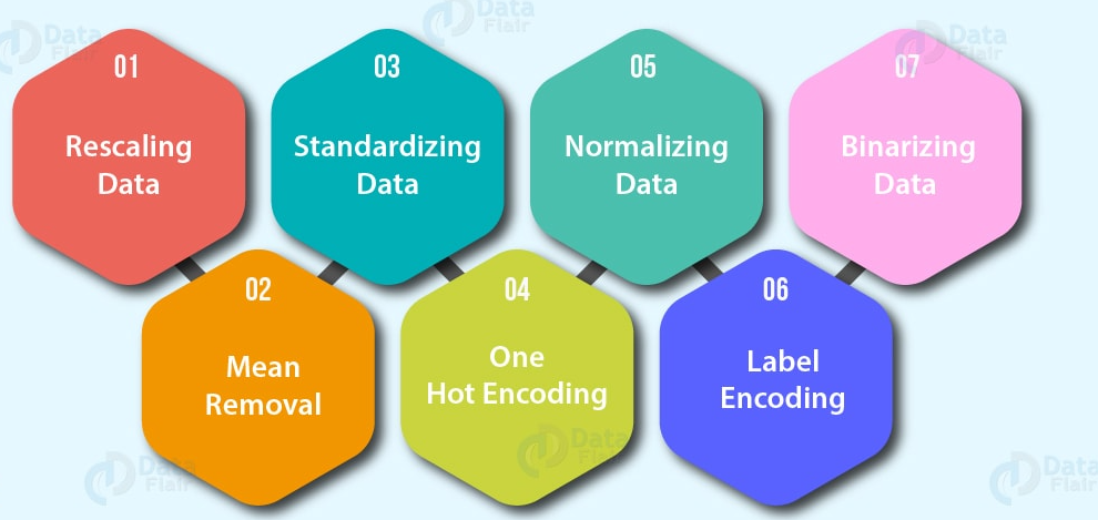
•  Feature encoding (turning values into numbers). A machine learning model
  requires all values to be numerical)

• One hot encoding: Turn all unique values into lists of 0’s and 1’s where the target value is 1 and the rest are 0’s. For example, when a car colors green, red blue, a green, a car’s color future would be represented as [1, 0, and 0] and a red one would be [0, 1, and 0].

•  Label Encoder: Turn labels into distinct numerical values. For example, if your target variables are different animals, such as dog, cat, bird, these could become 0, 1, and 2, respectively.

• Embedding encoding: Learn a representation amongst all the different data points. For example, a language model is a representation of how different words relate to each other. Embedding is also becoming more widely available for structured (tabular) data.

• Feature normalization (scaling) or standardization: When you’re numerical variables are on different scales (e.g. number_of_bathroom is between 1 and 5 and size_of_land between 500 and 20000 sq. feet), some machine learning algorithms don’t perform very well. Scaling and standardization help to fix this.

•  Feature engineering: transform data into (potentially) more meaningful representation by adding in domain knowledge

1. Decompose
2. Discretization: turning large groups into smaller groups
3. Crossing and interaction features: combining two or more features
4. The indicator features: using other parts of the data to indicate something potentially significant

• Feature selection: selecting
  the most valuable features of your dataset to model. Potentially reducing overfitting and training time(less overall data and less redundant data to train on) and improving accuracy.

1. Dimensionality reduction: A common dimensionality reduction method, PCA or principal component analysis taken a large number of dimensions (features) and uses linear algebra to reduce them to fewer dimensions. For example, say you have 10 numerical features, you could run PCA to reduce it down to 3.
2. Feature importance (post modelling): Fit a model to a set of data, then inspect which features were most important to the results, remove the least important ones.
3. Wrapper methods such as genetic algorithms and recursive feature elimination involve creating large subsets of feature options and then removing the ones which don’t matter.

•  Dealing with imbalances: does your data have 10,000 examples of one class but only 100 examples of another?

1. Collect more data (if you can)
2. Use the scikit-learn-contrib imbalanced- learn package
3.  Use SMOTE: synthetic minority over-sampling technique. It creates synthetic samples of your minor class to try and level the playing field.
4. A helpful paper to look at is “Learning from imbalanced Data”.

• Data splitting

1. Training set (usually 70-80% of data): Model learns on this.
2.  Validation set (usually 10-15% of data): Model hyperparameters are tuned on this
3. Test set (usually 10-15% of data): Models’ final performance is evaluated on this. If you have done it right, hopefully, the results on the test set give a good indication of how the model should perform in the real world. Do not use this dataset to tune the model.

3. Train model on data( 3 steps: Choose an algorithm, overfit the model, reduce overfitting with regularization)

• Choosing an algorithms 

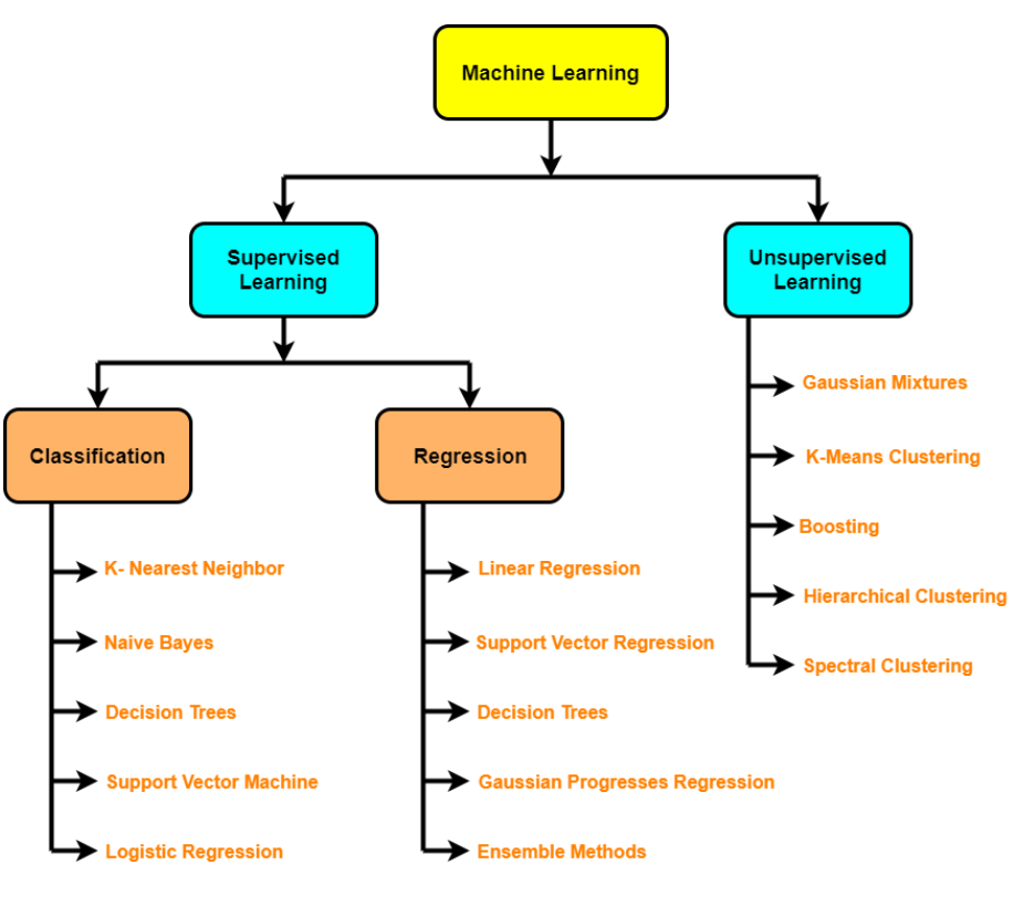
1.  Supervised algorithms – Linear Regression, Logistic Regression, KNN, SVMs, Decision tree and Random forests, AdaBoost/Gradient Boosting Machine(boosting)
2.  Unsupervised algorithms- Clustering, dimensionality reduction( PCA, Autoencoders, t-SNE), An anomaly detection

•  Type of learning 

1.  Batch learning
2.  Online learning
3. Transfer learning
4.  Active learning
5. Ensembling

•  Underfitting – happens when your model doesn’t perform as well as you’d like on your data. Try training for a longer or more advanced model.

• Overfitting– happens when your validation loss starts to increase or when the model performs better on the training set than on the test set.

1. Regularization: a collection of technologies to prevent/reduce overfitting (e.g. L1, L2, Dropout, Early stopping, Data augmentation, Batch normalization)

• Hyperparameter Tuning –  run a bunch of experiments with different settings and see which works best

4. Analysis/Evaluation

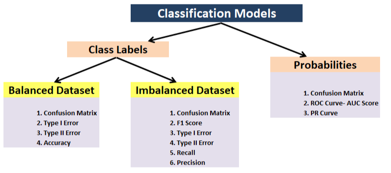
• Evaluation metrics

1. Classification- Accuracy, Precision, Recall, F1, Confusion matrix, Mean average precision (object detection)
2.  Regression – MSE,MAE,R^2
3. Task-based metric – E.g. for the self-driving car, you might want to know the number of disengagements

• Feature importance 
• Training/inference time/cost 
• What if tool: how does my model compare to other models? 
• Least confident examples: what does the model get wrong? 
• Bias/variance trade-off

5. Serve model (deploying a model) 

•  Put the model into production and see how it goes.
•  Tools you can use: TensorFlow Servinf, PyTorch Serving, Google AI Platform, Sagemaker
•  MLOps: where software engineering meets machine learning, essentially all the technology required around a machine learning model to have it working in production

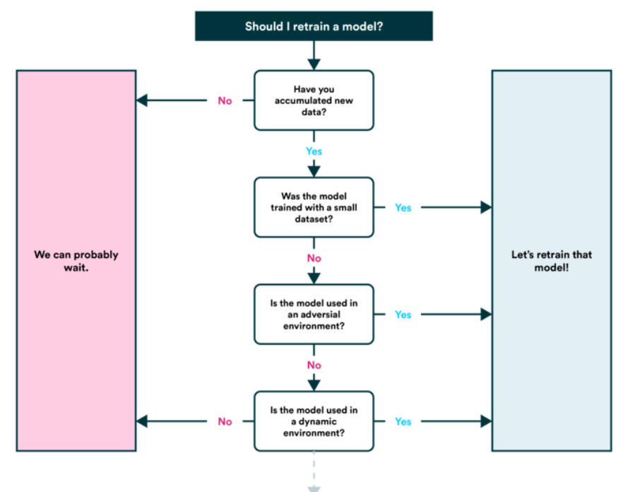
6. Retrain model

• See how the model performs after serving (or before serving) based on various evaluation metrics and revisit the above steps as required (remember, machine learning is very experimental, so this is where you’ll want to track your data and experiments.

•  You’ll also find your model’s predictions start to ‘age’ (usually not in a fine-wine style) or ‘drift’, as in when data sources change or upgrade(new hardware, etc.). This is when you’ll want to retrain it.

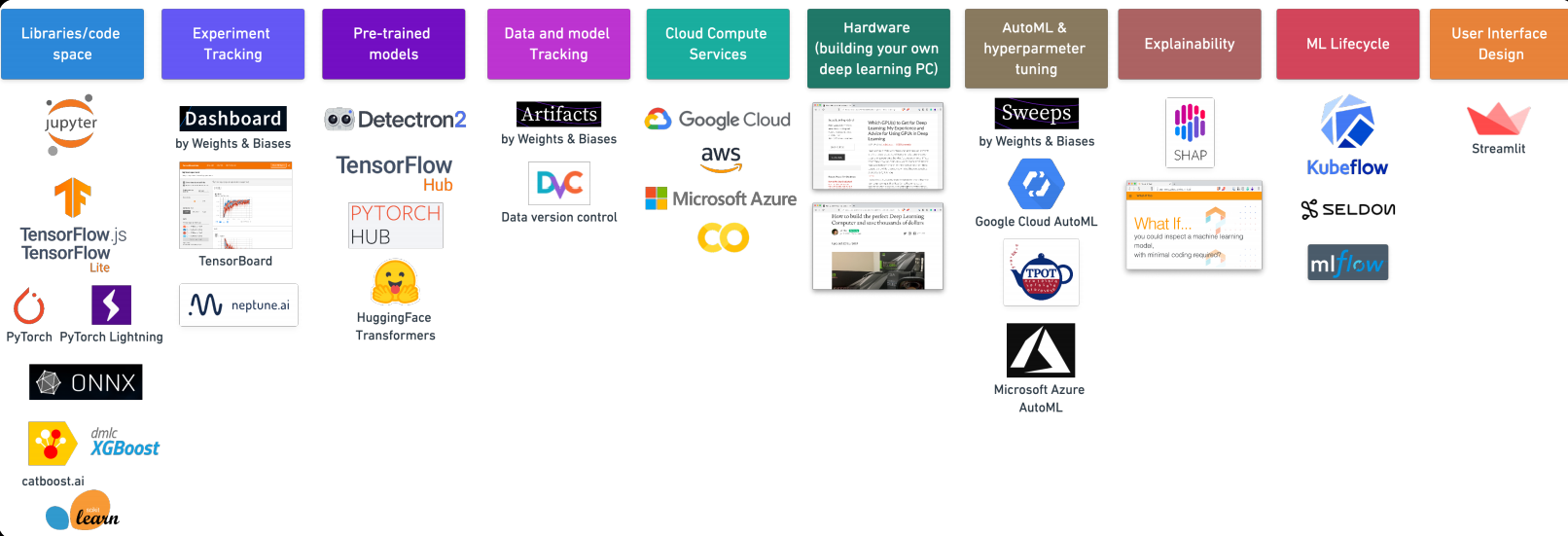
7. Machine Learning Tools

 

Thanks for reading this. If you like this article then please share it with your friends. In case of any suggestion/doubt comment below.

Email id: [email protected]

Follow me on LinkedIn: LinkedIn

Akshay Gupta

16 Apr 2021