Introduction
Most Kaggle-like machine learning hackathons miss a core aspect of a machine learning workflow – preparing an offline evaluation environment while building an ML product.
Getting to a stage where we have a clean train/test data split along with a machine learning metric to optimize usually takes much more effort than actually training a machine learning model. I’ve personally experienced a reality check when I started working as an ML engineer, after having spent a lot of time training models on proctored datasets.
In this blog post, I want to address one key component of designing an offline evaluation environment – creating a test set on which you can not only estimate ML performance metrics like accuracy, precision, recall, but also product metrics like click rates, revenue, etc.
We will use a causal inference based technique called counterfactual evaluation and understand it using an intuitive example from the industry and then dive into Python and simulate a real-world scenario!
Table of Contents
- Evaluating a Machine Learning Model Offline verses in Production
- Consider an Advertising Example
- Building and Setting up the Causal Graph
- Modeling Interventions
- Simulation of the Counterfactual Analysis (using Python)
Evaluating a Machine Learning Model Offline versus in Production
Developing and deploying a machine learning model in production typically starts with deploying a baseline or even heuristic-based model online, i.e. using it to make decisions on live traffic. This helps both in collecting the data to train a more sophisticated model and acts as a good performance benchmark.
This is followed by creating a train/validation/test dataset and training a model offline, So far, the model is not yet being used to make decisions impacting the end-user. Once we have a model, it’s common practice to deploy it online and run A/B tests to compare it with the heuristic model. We follow a similar process when iterating on an existing machine learning model in production.
One of the big challenges in this process is the validation of the offline model and deciding which model to try out online.
- If an offline model has a better offline machine learning metric like Area Under the Curve (AUC) than its production counterpart, is it necessarily better for business?
- Does a higher offline ML metric imply an improvement in business metrics?
- How much improvement in the offline ML metric is good enough to justify the deployment of a new model or running an A/B test?
These are some of the common questions which torment machine learning practitioners in their daily jobs, especially when building user-facing machine learning products. Some common scenarios behind these concerns are:
- Machine learning applications are trying to drive a product that is judged by business metrics like click rates, revenue, engagement, etc. These are dependent on user feedback/interaction in some form, which is hard to estimate offline
- Machine learning models are typically deployed along with some business heuristics which control how the model output translates to product action, such as diversity and also bias considerations during the content recommendation
- Many applications chain predictions from multiple models to take action. For example, the decision of which ad to show could depend on ML models for click rate predictions and demand forecasts along with business constraints like inventory and user eligibility
In such scenarios, typical machine learning metrics like accuracy, AUC-ROC, precision-recall, etc. for individual models are generally not enough to tell whether an offline model is a significant improvement over the model in production. A/B tests are typically used for such evaluation, but they are expensive to run both in terms of cost and time.
Counterfactual evaluation techniques, inspired by causal inference literature, provide a methodology of using production logs to estimate online metrics like click rate, revenue, etc. These act as good intermediate steps and help filter out offline models and select the right candidates for A/B testing, thus allowing us to explore a wide range of models offline.
Consider an Advertising Example
Let’s take an example from the advertising world to understand this better. Consider two sides of the following scenario:
- User side: A user visits a website and receives an ad; if the user likes the ad, they click on the ad, otherwise, they do not
- Business side: A machine learning system receives a request with current user context and picks an ad to display
This system can be defined using the following variables:
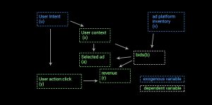
- user-intent (u): A user visits the website with some intent (example – user visits amazon.com to buy a shoe)
- user-context (x): User starts browsing on the website and their activity is packaged as a context vector
- ad inventory (c): Inventory of all ads available to show
- bids (b): A system which bids a price per click for ads from the ad inventory
- selected_ad (a): A final ad selected based on the bids and click estimates
- user action (y): Binary. 1 if the user clicks on the shown ad and 0 otherwise
- revenue (z): Some form of revenue ($$) generated from the interaction
Building and Setting Up the Causal Graph
What is a causal graph in the first place? This is how Wikipedia defines them:
“Causal graphs (also known as path diagrams, causal Bayesian networks or DAGs) are probabilistic graphical models used to encode assumptions about the data-generating process.”
The system with the above variables can be depicted as a causal graph like this:
From this graph, we can observe the dependence/relationship between different variables:
- u, v are independent variables, also known as exogenous variables
- x = f(u)
- b = f(x,v)
- a = f(x,b)
- y = f(a,u)
- z = f(y,b)
With this understanding, we can model the join probability of the entire system as a probabilistic generative model:
where w is the set of all variables.
Intuitively, we started with independent variables and then chained more variables together following the graph, while conditioning on the variables known at the time of determining a new variable. Note that this is an acyclic graph, i.e. if a causes b, then there is no causal path from b to a.
Isolation Assumption for the Causal Graph
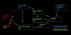
Before moving forward, let’s understand one of the core assumptions of this model. Like any causal graph, this graph assumes that the exogenous variables don’t have any backdoor path into the network, i.e. there is no common cause between the exogenous variables (u, v) and other variables in the network.
For example, suppose an external cause (e) exists which modifies the causal graph as:
In this case, the causal path represented in red is backdoor paths which invalidate the previously-defined system of equations. Another way of stating this assumption is that saying we assume all observations of exogenous variables are independently sampled from an unknown but fixed joint distribution. This is the isolation assumption.
Most causal graphs make this assumption. Since not all expected causes can be measured/modeled, we should try to measure the most impactful events. It is important to be mindful of this assumption while analyzing results.
Modeling Interventions
The causal graph and the system of equations allow us to modify a single element of the graph and estimate the impact on a metric defined on a downstream event.
Let’s say click rate is the business metric we’re trying to maximize. Click rate is defined as the proportion of advertisements clicked by users, across user sessions. Suppose we have a production system running and now we develop a new model for selecting an ad, i.e. we have a new way of implementing variable
a. We want to estimate the click rate of this model as compared to the production model.
This system of equations allows us to model interventions as algebraic manipulations i.e. we can change some interim distributions and model a different output for a given input.
Counterfactual Analysis – Evaluating a Hypothetical Model Deployment
Now, let’s dive into counterfactual analysis principles and try to solve the modeling intervention posed above.
What is Counterfactual?
The question – what would happen if we replace a current model M with a new model M’ – is counterfactual in the sense that we are not actually making the change and impacting user experience. We are just trying to estimate business metrics in the scenario if we were to hypothetically deploy the model M’.
An Analogy to Traditional Machine Learning
Let’s try to compare this scenario with a traditional supervised learning scenario.
While training models in a supervised learning setting, we use some independent variables x and true labels y, then we try to estimate y as y’ = f(x). y’ is kind of a counterfactual estimate of what would happen if, instead of the system generating the data, the model f(x) was used.
Then, we define a loss function and optimize the model. All of this works because f(x) is fully defined, which is not the case in our problem (i.e. there is no way to know how a user would have interacted if a different ad would be shown). Thus, we need some workaround so that we can estimate the metric without fully defining each component of the system.
Markov Factor Replacement for Counterfactual Analysis
Next, let’s try to perform algebraic manipulations in our system of equations. Say we have a new model M’ for the selection of an ad given bids. This will impact just one component of the equation:
The join distribution of the resulting system will be:
Note that only one distribution has changed. The click rate of the system can be defined as the expectation of click per impression:
Intuitively, this can be understood as an average of the clicks occurring in different context-action scenarios, represented by w, weighted by the probability distribution of w, which is a function of the user activity and production model M.
For a new model M’, the click rate would be:
To determine the click rate for a new model M’, we can simply adjust the probability distribution using the new model M’ given the same inputs from user activity. This can be rewritten as:
Assuming throughout the domain of w.
Using the law of large numbers, we can approximate as:
Observe how we have eliminated most of the components of the system from the final estimate. This is super powerful, because now we don’t need to fully define the joint distribution for the new model M’, but only the parts impacted by the intervention/change. This is typically easy to determine as the intervention is controlled.
This idea can be generalized for any given metric , the counterfactual estimate of an offline model M’ giving a probability distribution
. This can be determined using log data with probability distribution
as:
Intuition for the Marko Factor Replacement
Let’s try to understand this concept with a small example. Suppose there are 5 data points:
| context | p(M) | y | p(M’) |
|---|---|---|---|
| w1 | 0.8 | 1 | 0.3 |
| w2 | 0.6 | 1 | 0.5 |
| w3 | 0.2 | 0 | 0.4 |
| w4 | 0.1 | 0 | 0.3 |
| w5 | 0.7 | 1 | 0.6 |
Here,
- Each row is a context where an ad was shown
- p(M) is the logged probability of showing the ad by the production model M
- p(M’) is the probability that an offline model M’ will show the same ad
- y is the user action, 1 if clicked 0 if not
We can see that the production model usually has a high probability of showing when the user clicked, hence it’s a better model.
The estimator will give a similar inference. Thus, we are able to get back our intuitive ordering of models from the counterfactual estimate.
Constraints / Practical Considerations
If we carefully observe the final equation, it puts a constraint on the model being evaluated. The model has to be probabilistic in nature, and we can determine the probability of taking the exact same action which the logging model took, which may not always be trivial.
Suppose we only have the final action a’ taken by the new model for each log entry. Then, we can also re-write the same equation by taking inspiration from propensity score matching based approaches [2]:
Intuitively, you can understand this as considering the new model to be probabilistic and making wherever the new model takes a different action than the logged model.
In practice, using the matching approach works if we have a fewer number of actions and we expect to match a fair number of actions from the logged dataset. However, there are numerous scenarios like a recommendation, information retrieval, or multi-arm bandits where we may not have sufficient data to get enough matches for reliable estimates resulting in high variance.
Please note that for the sake of simplicity, we will be not be discussing variance considerations in this article, but feel free to read more in references [1] [2] I have provided at the bottom of this article.
Simulation of the Counterfactual Analysis (using Python)
At this point, you would have developed some intuitive and mathematical understanding of counterfactual analysis. Let’s take it a step further using a simulated example, similar to the one we’ve been working with. Suppose:
- We have 3 ads in inventory, valid for all users
- We simulate N number of user contexts, i.e. N different user scenarios, each with an independent click probability on one of the ads
- We collect some online data by serving ads randomly to users in different contexts and observing click behavior. Random serving is a good way to collect unbiased online data to evaluate online models and should be adopted when possible
1. Data Preparation
Let’s simulate some logged data which is similar to something coming from a production system. Let’s import the necessary packages first.
User Contexts
We’ll start by defining 10,000 user context (x) ids and define a probability distribution on their occurrence, i.e. some contexts are more likely to repeat than others.
Click Rate Per Context
Let’s define 3 ads in our inventory. For the sake of simplicity, let’s say the click rate for a given ad in a given context can be one of:
- Low: 10%
- Medium: 40%
- High: 60%
Then, we can randomly assign which of the ads is low/medium/high and in which context. The idea is that a good model will pick the high-interaction ad in a given context more often than the low-interaction ad.
2. Random Data Collection
Now, let’s simulate 100,000 iterations where one of the 10,000 user contexts is given as input to the model, a random ad is served and based on the click prior to that ad in that context, the action of click or no click is sampled.
The idea here is to generate data similar to production logs of any model, the difference being that we are simulating the user side.
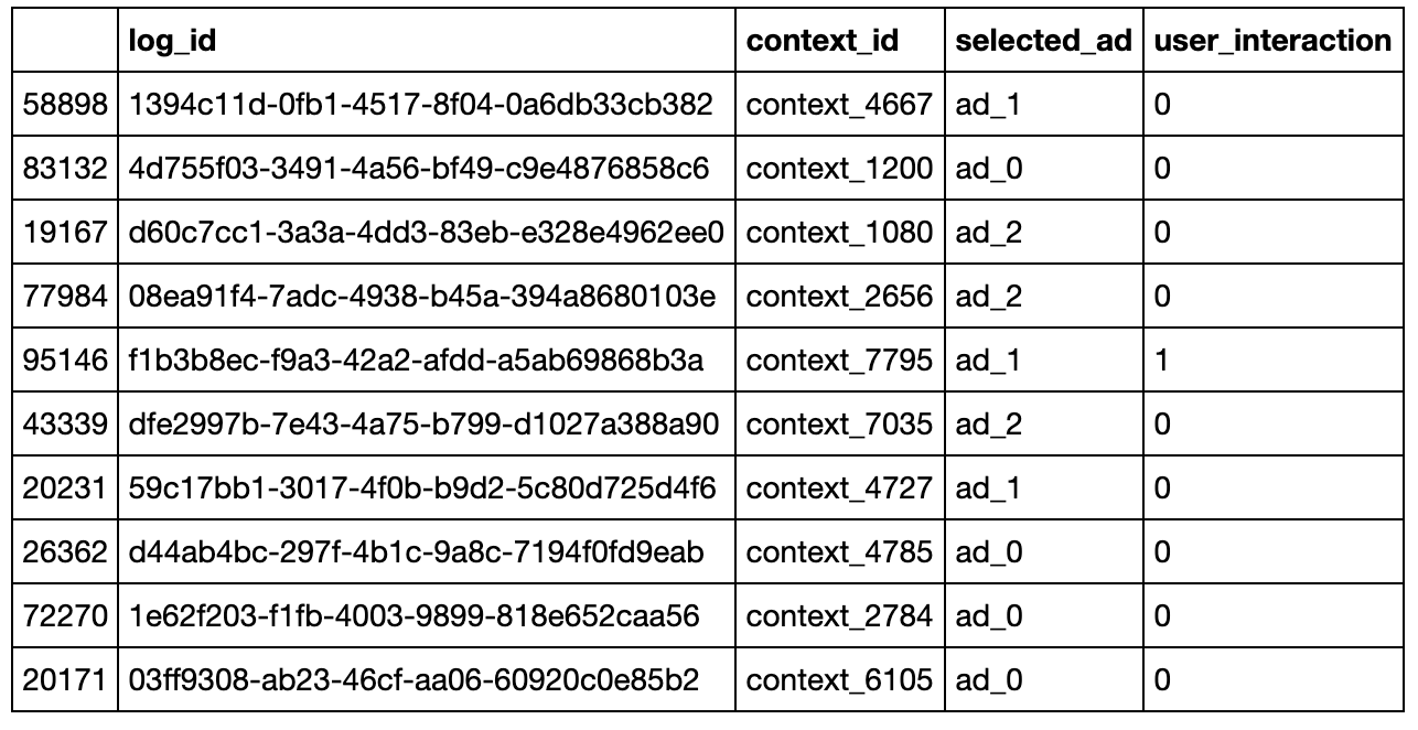
The simulated data will contain four columns:
- log_id: represents each logged row
- context_id: represents the user context from our list of 10,000 contexts
- selected_ad: the ad shown by the production model
- user_interaction: binary 1 if the user interacted and 0 otherwise
To recap, each row in this simulated log data represents an instance where:
- a user visited a website with some intent and generated a user context (x) denoted by context_id.
- a production model (random in this case) selected an ad to show to the user
- the user interaction was observed and logged
3. New Model Estimation
Define Models
Next, let’s define some models for which we can establish an intuition of order of performance on click rate. This will allow us to simulate offline model predictions, use counterfactual estimation to get metrics and compare them with expected results.
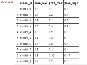
One way to do so is to set priors on the likelihood of picking the low/med/high ad using a vector [p_low, p_med, p_high] for a given context. We can intuitively say that the models with a higher likelihood of picking more performant ads for a context will work better. Note that this is not how an actual model would work because we wouldn’t know the click rate prior; think of these as models that have learned these priors with different levels of accuracy.
Here’s a group of 10 models with increasing expected performance:
For clarification, let’s see this as a data frame:
One nice feature of defining a model in this way is that we can actually calculate the expected click rate of each model. Since a model is a set of priors on picking a low/med/high ad, and we have already fixed the interaction rates of low/med/high ads, we can just take a dot product to estimate the click rate:
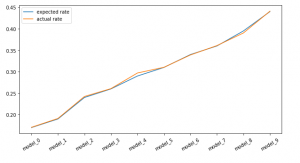
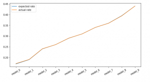
Output: array([0.17 , 0.19 , 0.24 , 0.26 , 0.29 , 0.31 , 0.34 , 0.36 , 0.395, 0.44 ])
We can see that expected click rates are in the order that we expect. Now we’ll try to sample ad selections using each policy and use the counterfactual technique learned above to see if we can estimate these click rates using only the logged data and sampled outcomes from each model.
Estimate Click Rate: Propensity Matching
First, let’s use the propensity matching estimate:where:
: user interaction
: action suggested by new model
: action taking by production model
: logged probability of the production model (random serving)
We can see that for each log entry we’ve computed the ad selection from all new models.
Estimate Click Rate: Propensity Weighting
First, let’s use the propensity matching estimate:
Here:
: user interaction
: selection probability of the offline model being evaluated
: logged probability of the production model (random serving)
We can see that for each log entry, we’ve computed the probability of the same ad selection as a production model from all new models.
Conclusion
We saw that in the case of both the estimators, we were able to estimate the right click rate for each model. In other words, had we not known the actual order of performance of each model, this technique would help us pick the right model just from the predicted outcomes of each model on the logged entries.
It is important to note that in this simulated example, we were able to retrieve the exact click rates. In practice, however, there could be various sources of noise and we may not get the exact numbers back. However, we could aim for three properties, in order of increasing importance, when evaluating offline evaluation methodologies:
- Directionality:
- if the online metric for model A > model B, then the counterfactual metric for model A > model B.
- Rate of Change:
- if the online metric for model A is 10% more than model B, then the counterfactual metric is also higher by a similar amount
- Exact Values:
- the online and counterfactual metrics are very close in absolute value, as our example (this is ideal case)
Did you find this helpful? Can you think of scenarios in your daily job where this technique could be useful? Do you see any limitations of this approach not highlighted here? Feel free to drop comments with feedback/criticism/questions; I would love to discuss more.
References/Additional Reading
This article is heavily influenced by [1] and [2]. If you are interested in digging further, [3] [4] [5] are interesting reads with more applications of similar context:
- Counterfactual Reasoning & Learning Systems
- Counterfactual Estimation and Optimization of Click Metrics for Search Engines
- The Self-Normalized Estimator for Counterfactual Learning
- Unbiased Offline Evaluation of Contextual-bandit-based News Article Recommendation Algorithms
- Off-policy evaluation for slate recommendation
If you want to reuse some of the code in here, you could use this jupyter notebook version on the writeup on git.


