Introduction
As data scientists and machine learning practitioners, we come across and learn a plethora of algorithms. Have you ever wondered where each algorithm’s true usefulness lies? Are most machine learning techniques learned with the primary aim of scaling a hackathon’s leaderboard?
Not necessarily. It’s important to examine and understand where and how machine learning is used in real-world industry scenarios. That’s where most of us are working (or will eventually work). And that’s what I aim to show in this part 3 of our popular series covering the fast.ai introduction to machine learning course!
We covered a fairly comprehensive introduction to random forests in part 1 using the fastai library, and followed that up with a very interesting look at how to interpret a random forest model. The latter part is especially quite relevant and important to grasp in today’s world.
In this article, we will first take a step back and analyze machine learning from a business standpoint. Then we’ll jump straight back to where we left off part 2 – building a random forest model from scratch. I encourage you to hop back to the previous posts in case you need to refresh any concept, and carry that learning with you as we move forward.
Table of Contents
- Introduction to Machine Learning: Lesson 6
- Machine Learning Applications in Business
- Random Forest Interpretation Techniques
- Introduction to Machine Learning: Lesson 7
- Building a Random Forest from Scratch in Python
Introduction to Machine Learning: Lesson 6
Having learned the basic underlying concept of a random forest model and the techniques used to interpret the results, the obvious follow-up question to ask is – where are these models and interpretation techniques used in real life? It’s all well and good knowing the technique, but if we don’t know where and when to apply it, it feels like a wasted effort.
Jeremy Howard answers this question in Lesson #6, where he explains how a random forest model can be used to interpret and understand the data. This lesson is also a walkthrough covering all the techniques we have learned in the previous two articles.
In this section, we will look at various sectors where machine learning has already made it’s presence felt and is being implemented successfully.
The business market, as explained by Jeremy, can broadly be divided into two groups – horizontal and vertical. We will look at these individually, but first, let’s understand the most important steps involved in designing a machine learning model.
There are broadly four steps we follow for doing this. These collectively form the “drivetrain approach”, as explained by Jeremy in his paper: Designing Great Data Products.
Step 1: Define the Objective
Before diving into the challenge and building a machine learning model, one must have a clear, well-defined objective or an end goal in mind. This may vary depending on what the organization is trying to achieve. A couple of examples are given below:
- Selling more number of books/products
- Reduce the number of customers that leave/attrite
Step 2: Levers
Levers are the inputs that can be controlled, or some changes the organization can make, to drive the objective defined in step 1. For instance, to ensure that the customers are satisfied:
- A seller can give special offers on his products
- Give free pen or other merchandise on a purchase of more than $20
A machine learning model cannot be a lever, but it can help the organization identify the levers. It’s important to understand this distinction clearly.
Step 3: Data
The next step is to find out what data can be helpful in identifying and setting the lever that the organization may have (or can collect). This can be different from the data already provided or collected by the organization earlier.
Step 4: Predictive models
Once we have the required data that can be helpful in achieving the above defined goal, the last step is to build a simulation model on this data. Note that a simulation model can have multiple predictive models. For example, building one model identifying what items should be recommended to a user, and another model predicting the probability that a user buys a particular product on a recommendation. The idea is to create an optimization model, rather than a predictive model.
You can read the paper I linked above to understand these steps in more detail. We’ll move on to understand the applications of machine learning from the industry and business point-of-view.
Machine learning Applications in Business
As we alluded to earlier, we can divide the business market broadly into two groups – horizontal and vertical. I will elaborate on each in this section to give you an industry-level perspective on things.
Horizontal Market
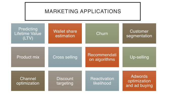
Horizontal markets are usually defined by demography (can be common across different kinds of business), which is broadly everything involving marketing. Here is a group of marketing applications where machine learning can (and is) be used.
Taking the example of ‘Churn’, the goal is to determine who is going to leave or attrite. Suppose an organization has a churn model that predicts which employee is going to leave and what can be changed so that the number of employees leaving is reduced.
Once the end goal is defined, we can make a list of things that can be changed in order to decrease the number of people who are leaving the organization and collect whatever data we need to build a model.
Then we can create a random forest model and use the interpretation techniques we learned previously. For instance, the feature importance aspect from the random forest model can help us understand which features matter the most. Or the pdp plot visualization can be useful in determining how a particular change will affect the target variable (aka probability of an employee attriting).
Vertical Market
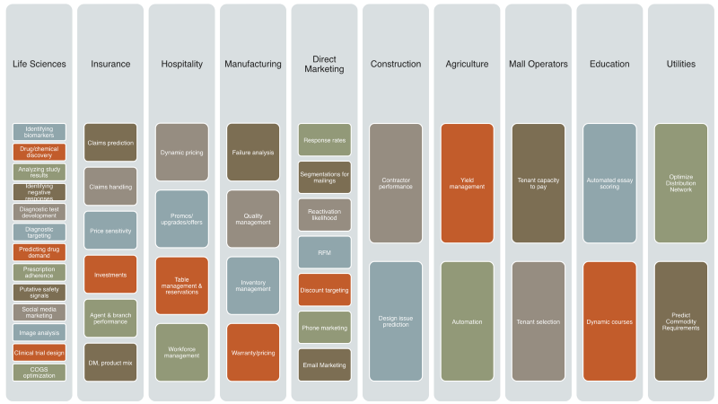
Vertical market refers to a group of businesses sharing the same industry, such as education, healthcare, aerospace, finance, etc. Below are a couple of examples where machine learning is being used in such cases:
- Healthcare: A ML model can be used to predict the risk of readmission for a patient. Based on the data about the patient, such as his/her age, BP, platelet count, heart rate, etc., the model can predict the probability that the patient will be readmitted and can be used to find the exact reason behind it.
- Aircraft scheduling: A model can be used to predict the chances of the delayed arrival for a flight which is useful for organizing people and deciding gate management.
It’s a good exercise to discuss the applications of machine learning in various domains and answer the following questions for each:
- What are the possible applications of machine learning in each domain?
- What is the objective and what will be the predictions?
- What kind of data will be required and which ML model can be used for the task?
Our discussion so far would have given you a fair idea about the plethora of machine learning applications in the industry. We’ll do a quick review of the random forest interpretation techniques and then continue building the random forest model from scratch after that.
Random Forest Interpretation Techniques
We’ll quickly recap these techniques since we have covered them in part 2. For a more detailed explanation, you can take a look at this article:
Standard deviation
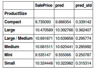
We calculated the standard deviation of the predictions (for each level in Enclosure and ProductSize) to figure out which categories are being wrongly predicted by the model and why.
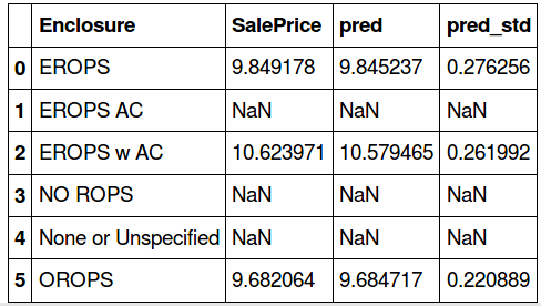
We found that for categories with a low value count, the model is giving a high standard deviation. So there are higher chances that the predictions for categories with a larger value count are more accurate (since the model is trained well for these categories). Makes sense, right?
Feature Importance
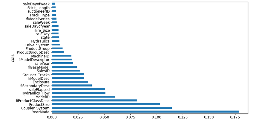
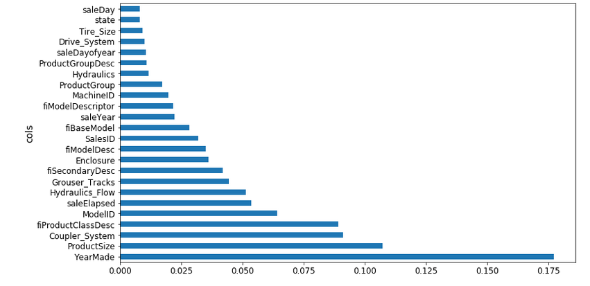
Feature importance is basically determining how important a feature is in predicting the target variable. The top 30 variables for the random forest model are the following:
As it is evident from the above plot, YearMade is the most important variable. This makes sense because the older the vehicle, the lesser the saleprice. The model performance improved when the less important features were removed from the training set. This, as you can imagine, can be really helpful in understanding the data and variables. Additionally, we can use one-hot encoding to create columns for each level and then calculate the feature importance:
Partial Dependence Plot (PDP)
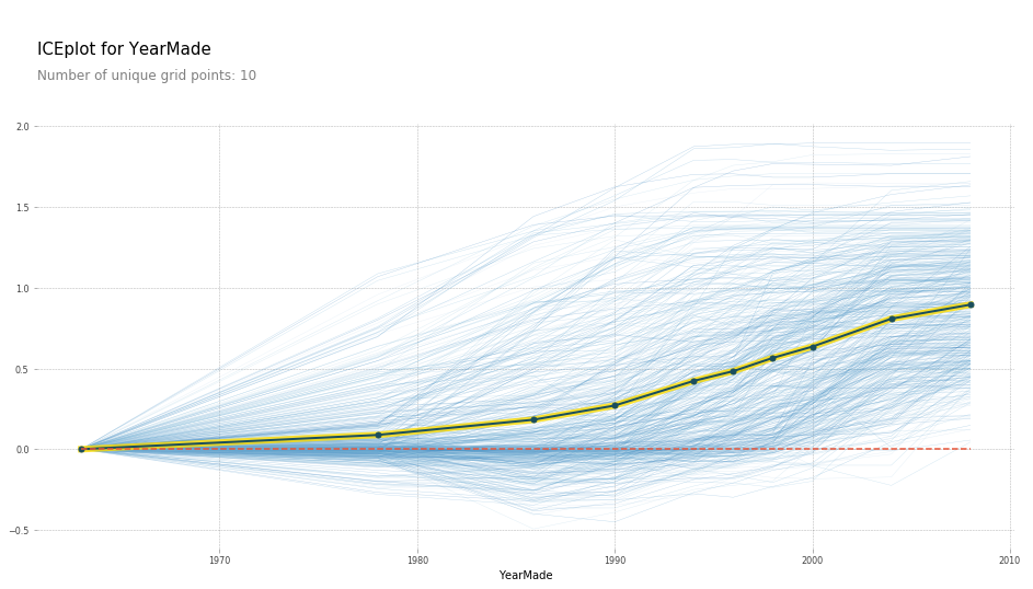
Partial dependence is used to understand the dependence of features on the target variable. This is done by predicting the target for each row, keeping a variable constant. For instance, predicting saleprice for each row when YearMade is 1960, then for YearMade 1961, and so on. The result would be a plot like this:
Tree Interpreter
The tree interpreter is used to evaluate the predictions for each row using all the trees in the random forest model. This also helps us understand how much each variable contributed to the final prediction.
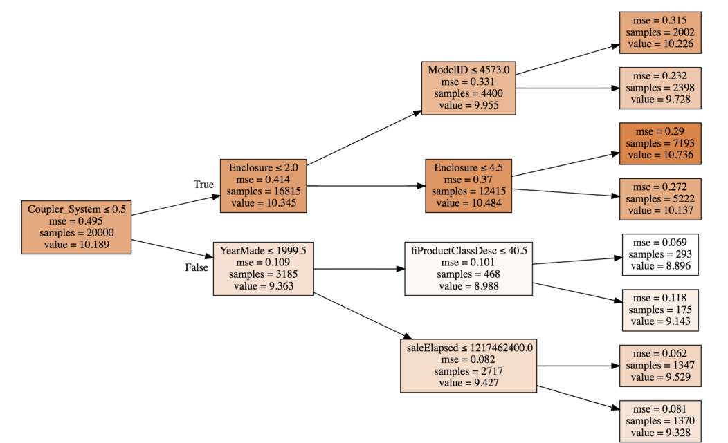
Before we understand how the contribution for multiple trees is calculated, let’s take a look at a single tree:
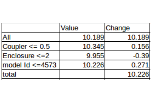
The value of Coupler_System<=5 is 10.189, for Enclosure<=2 is 2.0, and model_id comes out to be 9.955 (considering only the top most path for now).
The value for Enclosure <=2 is not only because of the feature Enclosure, but a combination of Coupler_System and Enclosure. In other words, we can say that Coupler_System interacted with Enclosure with a contribution of 0.156. Similarly, we can determine the interaction importance between features.
Now we can use the average of all the trees in order to calculate the overall contribution by each feature. For the first row in the validation set, below are the contributions by each variable:
[('ProductSize', 'Mini', -0.54680742853695008),
('age', 11, -0.12507089451852943),
('fiProductClassDesc',
'Hydraulic Excavator, Track - 3.0 to 4.0 Metric Tons',
-0.11143111128570773),
('fiModelDesc', 'KX1212', -0.065155113754146801),
('fiSecondaryDesc', nan, -0.055237427792181749),
('Enclosure', 'EROPS', -0.050467175593900217),
('fiModelDescriptor', nan, -0.042354676935508852),
('saleElapsed', 7912, -0.019642242073500914),
('saleDay', 16, -0.012812993479652724),
('Tire_Size', nan, -0.0029687660942271598),
('SalesID', 4364751, -0.0010443985823001434),
('saleDayofyear', 259, -0.00086540581130196688),
('Drive_System', nan, 0.0015385818526195915),
('Hydraulics', 'Standard', 0.0022411701338458821),
('state', 'Ohio', 0.0037587658190299409),
('ProductGroupDesc', 'Track Excavators', 0.0067688906745931197),
('ProductGroup', 'TEX', 0.014654732626326661),
('MachineID', 2300944, 0.015578052196894499),
('Hydraulics_Flow', nan, 0.028973749866174004),
('ModelID', 665, 0.038307429579276284),
('Coupler_System', nan, 0.052509808150765114),
('YearMade', 1999, 0.071829996446492878)]
Just a reminder that the calculation behind the values generated has been covered in the previous post.
Extrapolation
For this particular topic, Jeremy performs live coding during the lecture by creating a synthetic dataset using linespace. We have set the start and end points as 0 and 1.
%matplotlib inline
from fastai.imports import *
from sklearn.ensemble import RandomForestRegressor
x=np.linspace(0,1)
x
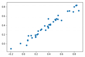
The next step is to create a dependent variable. For simplicity, we assume a linear relationship between x and y. We can use the following code to generate our target variable and plot the same:
Python Code:
We’ll convert our 1D array into a 2D array which will be used as an input to the random forest model.
x1=x[...,None]
Out of the 50 data points, we’ll take 40 for training our random forest model and keep the remaining 10 to be used as the validation set.
x_trn, x_val = x1[:40], x1[40:]
y_trn, y_val = y[:40], y[40:]
We can now fit a random forest model and compare the predictions against actual values.
m = RandomForestRegressor().fit(x_trn, y_trn)
plt.scatter(y_trn, m.predict(x_trn))
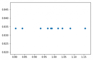
The results are pretty good, but do you think we’ll get similar results on the validation set? We have trained our model on the first 40 data points, the scale of which is actually very different from that of the validation set. So any new point that the random forest model tries to predict, it inevitably identifies that these points are closer to the highest of the given 40 points.
Lets have a look at the plot:
This confirms our hunch that random forest cannot extrapolate to a type of data that it has never seen before. It’ll basically give you the average of the data it has previously seen. So how should one deal with this type of data? We can potentially use neural nets which have proved to work better with such cases. Another obvious solution is to use time series techniques (which i have personnaly worked on and can confirm that they show far better results).
So to conclude lesson #6, we covered the necessary steps involved in building a machine learning model and briefly looked at all the interpretation techniques we learned in the previous article. If you have any questions on this section, please let me know in the comments below the article.
Introduction to Machine Learning: Lesson 7
We started learning how to build a random forest model from scratch in the previous article. We’ll take it up from where we left off in this section (lesson #7). By the end of this lesson, you’ll be able to build an end-to-end random forest model from the ground up on your own. Sounds pretty exciting so let’s continue!
We have discussed the random forest algorithm in detail – from understanding how it works to how the split points are selected, and how the predictions are calculated. We are now going to put our understanding into code form, one step at a time, i.e., creating a model that works with few features, smaller number of trees, and a subset of the data.
Note: Steps 1 to 6 have been covered in the previous article.
Step 1: Importing the basic libraries.
%load_ext autoreload
%autoreload 2
%matplotlib inline

from fastai.imports import *
from fastai.structured import *
from sklearn.ensemble import RandomForestRegressor, RandomForestClassifier

from IPython.display import display
from sklearn import metrics
Step 2: Read the data and split into train and validation sets.
PATH = "data/bulldozers/"

df_raw = pd.read_feather('tmp/bulldozers-raw')
df_trn, y_trn, nas = proc_df(df_raw, 'SalePrice')

def split_vals(a,n): return a[:n], a[n:]
n_valid = 12000
n_trn = len(df_trn)-n_valid

X_train, X_valid = split_vals(df_trn, n_trn)
y_train, y_valid = split_vals(y_trn, n_trn)

raw_train, raw_valid = split_vals(df_raw, n_trn)
Step 3: Take a subset of data to start with.
As I previously mentioned, we’ll take smaller steps, so here we pick only two features and work with them. If that works well, we can complete the model by taking all the features.
x_sub = X_train[['YearMade', 'MachineHoursCurrentMeter']]
Step 4: Define the set of inputs:
- A set of features – x
- A target variable – y
- Number of trees in the random forest – n_trees
- A variable to define the sample size – sample_sz
- A variable for minimum leaf size – min_leaf
- A random seed for testing
  def __init__(self, x, y, n_trees, sample_sz, min_leaf=5):
       np.random.seed(42)
       self.x,self.y,self.sample_sz,self.min_leaf = x,y,sample_sz,min_leaf
       self.trees = [self.create_tree() for i in range(n_trees)]
Step 5: Define a function that uses a sample of data (with replacement) and creates a decision tree over the same.
  def create_tree(self):
       rnd_idxs = np.random.permutation(len(self.y))[:self.sample_sz]
       return DecisionTree(self.x.iloc[rnd_idxs], self.y[rnd_idxs], min_leaf=self.min_leaf)
Step 6: Create a predict function. The mean of the predicted value from each tree for a particular row is returned as the final prediction.
  def predict(self, x):
       return np.mean([t.predict(x) for t in self.trees], axis=0)
Combining all the above functions, we can create a class TreeEnsemble.
class TreeEnsemble():
   def __init__(self, x, y, n_trees, sample_sz, min_leaf=5):
       np.random.seed(42)
       self.x,self.y,self.sample_sz,self.min_leaf = x,y,sample_sz,min_leaf
       self.trees = [self.create_tree() for i in range(n_trees)]

   def create_tree(self):
       rnd_idxs = np.random.permutation(len(self.y))[:self.sample_sz]
       return DecisionTree(self.x.iloc[rnd_idxs], self.y[rnd_idxs], min_leaf=self.min_leaf)

   def predict(self, x):
       return np.mean([t.predict(x) for t in self.trees], axis=0)
Step 7: Create a class DecisionTree. We call DecisionTree in the function create_tree, so let’s define it here. A decision tree would have a set of independent variables, a target variable, and the index values. For now, we have created only one decision tree (we can make it recursive later).
class DecisionTree():
  def __init__(self, x, y, idxs=None, min_leaf=5):
      if idxs is None: idxs=np.arange(len(y))
      self.x,self.y,self.idxs,self.min_leaf = x,y,idxs,min_leaf ##define x,y,index and minimum leaf size
      self.n,self.c = len(idxs), x.shape[1]  ##number of rows and columns
      self.val = np.mean(y[idxs])
      self.score = float('inf')
      self.find_varsplit()
Step 8: Determine the best split point. For every column, we use the function find_better_split to identify a split point and then return the column name, value, and score for the split.
  def find_varsplit(self):
      for i in range(self.c): self.find_better_split(i) #check for each column in the dataset

def find_varsplit(self):
       for i in range(self.c): self.find_better_split(i)

  @property
  def split_name(self): return self.x.columns[self.var_idx]

  @property
  def split_col(self):
      return self.x.values[self.idxs,self.var_idx]

  @property
  def is_leaf(self): return self.score == float('inf')

  def __repr__(self):
      s = f'n: {self.n}; val:{self.val}'
      if not self.is_leaf:
          s += f'; score:{self.score}; split:{self.split}; var:
                 {self.split_name}'
      return s
Step 9: Build our first model with 10 trees, a sample size of 1,000 and minimum leaf as 3.
m = TreeEnsemble(X_train, y_train, n_trees=10, sample_sz=1000,min_leaf=3)
m.trees[0]
For the first tree, the results are:
n: 1000; val:10.079014121552744
Let’s now fill the block that we left above in Step 8 – find_better_split. This is by far the most complicated part of the code to understand, but Jeremy has explained using a simple example in excel. I will explain it in an intuitive manner here.
For each variable, we split the points to the left and right node, and check the score for every value. The idea is to find a split point where we are able to separate more similar points together.
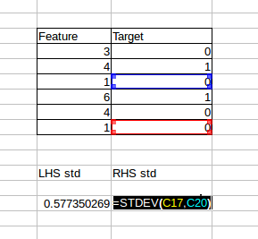
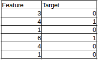
Consider the following example: we have two columns – an independent variable which we try to split on, and a binary target variable.
We will split at each value of the first column and calculate a standard deviation to identify how well we were able to classify the target. Let’s suppose the first split point is >=3, and then calculate the standard deviation.
We can take a weighted average of this value. Similarly, we can calculate for a split at 4, 6, 1 and so on. Let’s put this into code:
 def find_better_split(self, var_idx):
   x,y = self.x.values[self.idxs,var_idx], self.y[self.idxs]

   for i in range(self.n):
       lhs = x<=x[i]
       rhs = x>x[i]
       if rhs.sum()<self.min_leaf or lhs.sum()<self.min_leaf: continue
       lhs_std = y[lhs].std()
       rhs_std = y[rhs].std()
       curr_score = lhs_std*lhs.sum() + rhs_std*rhs.sum()
       if curr_score<self.score:
           self.var_idx,self.score,self.split = var_idx,curr_score,x[i]
If we try to print the results of the function for both the columns individually, we get the below result:
find_better_split(tree,1)
tree
n: 1000; val:10.079014121552744; score:681.0184057251435; split:3744.0; var:MachineHoursCurrentMeter
find_better_split(tree,0);
tree
n: 1000; val:10.079014121552744; score:658.5510186055949; split:1974.0; var:YearMade
Looks like YearMade 1974 is a better split point.
Step 10: Compare with the scikit-learn random forest. But keep in mind that there’s a tricky aspect here. While comparing the two models, both of them should have the same input. So let’s store the input that we have used in the random forest we just built.
ens = TreeEnsemble(x_sub, y_train, 1, 1000)
tree = ens.trees[0]
x_samp,y_samp = tree.x, tree.y
And now we build a model on this subset:
m = RandomForestRegressor(n_estimators=1, max_depth=1, bootstrap=False)
m.fit(x_samp, y_samp)
draw_tree(m.estimators_[0], x_samp, precision=2)
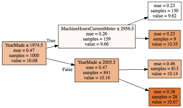
We see that the split here is on the column YearMade at year 1974.5, very similar to the results of our model. Not bad!
Step 11: There’s a problem with the code we have seen so far – can you recognize what it is? We need to optimise it! in the current format, we are checking the score for the split at each row, aka we are checking for a single value multiple times. Have a look at the example we used earlier:
The function will check the split points 4 and 1 twice because it actually works row-wise. It’s a good idea to optimise our code so as to reduce the computation time (not everyone has a top machine!). The idea is to sort column-wise and then check the score after the split for unique values only.
sort_idx = np.argsort(x)
sort_y,sort_x = y[sort_idx], x[sort_idx]
Also, to calculate the standard deviation, we define the following function:
def std_agg(cnt, s1, s2): return math.sqrt((s2/cnt) - (s1/cnt)**2)
We will need to keep a track of the count of data points on each side of the split along with the sum of square of the values. So we initialize the variables rhs_cnt, lhs_cnt, rjs_sum2 and lhs_sum2.
rhs_cnt,rhs_sum,rhs_sum2 = self.n, sort_y.sum(), (sort_y**2).sum()
lhs_cnt,lhs_sum,lhs_sum2 = 0,0.,0.
Adding all this up, the code looks like this:
tree = TreeEnsemble(x_sub, y_train, 1, 1000).trees[0]
def std_agg(cnt, s1, s2): return math.sqrt((s2/cnt) - (s1/cnt)**2)
def find_better_split_foo(self, var_idx):
x,y = self.x.values[self.idxs,var_idx], self.y[self.idxs]

sort_idx = np.argsort(x)
sort_y,sort_x = y[sort_idx], x[sort_idx]

rhs_cnt,rhs_sum,rhs_sum2 = self.n, sort_y.sum(), (sort_y**2).sum()
lhs_cnt,lhs_sum,lhs_sum2 = 0,0.,0.

for i in range(0,self.n-self.min_leaf-1):
  xi,yi = sort_x[i],sort_y[i]
  lhs_cnt += 1; rhs_cnt -= 1
  lhs_sum += yi; rhs_sum -= yi
  lhs_sum2 += yi**2; rhs_sum2 -= yi**2
  if i<self.min_leaf or xi==sort_x[i+1]:
    continue

  lhs_std = std_agg(lhs_cnt, lhs_sum, lhs_sum2)
  rhs_std = std_agg(rhs_cnt, rhs_sum, rhs_sum2)
  curr_score = lhs_std*lhs_cnt + rhs_std*rhs_cnt
  if curr_score<self.score:
    self.var_idx,self.score,self.split = var_idx,curr_score,xi
Ideally, this function should give the same results. Let’s check:
%timeit find_better_split_foo(tree,1)
tree
2.2 ms ± 148 µs per loop (mean ± std. dev. of 7 runs, 100 loops each)
n: 1000; val:10.079014121552744; score:658.5510186055565; split:1974.0; var:YearMade
Note that we created a new function (slightly changed the name from find_better_split to find_better_split_foo), and we need to use this in our DecisionTree class. The following command does it for us:
DecisionTree.find_better_split = find_better_split_foo
Step 12: Build our tree with more than one split.
In step 10, we compared the first level of our model with the scikit-learn random forest model. We will now create a full tree (which splits on both our features) and compare it again. Right now our find_varsplit function looks like this:
def find_varsplit(self):
      for i in range(self.c): self.find_better_split(i)
where we have defined find_better_split separately. We will update this function, so that it automatically checks for the leaf node and stores a list of indices in lhs and rhs after the split.
def find_varsplit(self):
  for i in range(self.c): self.find_better_split(i)
  if self.is_leaf: return
  x = self.split_col
  lhs = np.nonzero(x<=self.split)[0]
  rhs = np.nonzero(x>self.split)[0]
  self.lhs = DecisionTree(self.x, self.y, self.idxs[lhs])
  self.rhs = DecisionTree(self.x, self.y, self.idxs[rhs])

DecisionTree.find_varsplit = find_varsplit
We will again compare both the models. Previously, the max_depth was restricted to 1, and we will make it 2 here (we have only two features for now):
m = RandomForestRegressor(n_estimators=1, max_depth=2,  bootstrap=False)
m.fit(x_samp, y_samp)
draw_tree(m.estimators_[0], x_samp, precision=2)
And now look at our results:
tree = TreeEnsemble(x_sub, y_train, 1, 1000).trees[0]
tree
n: 1000; val:10.079014121552744; score:658.5510186055565; split:1974.0; var:YearMade
According to the image above, lhs should have 159 samples and a value of 9.66, while rhs should have 841 samples and a value of 10.15.
tree.lhs
n: 159; val:9.660892662981706; score:76.82696888346362; split:2800.0; var:MachineHoursCurrentMeter
tree.rhs
n: 841; val:10.158064432982941; score:571.4803525045031; split:2005.0; var:YearMade
Everything looks perfect so far! Going one level deeper into the tree, the left side of lhs should consist of 150 samples:
tree.lhs.lhs
n: 150; val:9.619280538108496; score:71.15906938383463; split:1000.0; var:YearMade
Great! We are able to build our own tree. Let’s create a function to calculate the predictions and then we’ll compare the r-square values.
Step 13: Calculate the final predictions. We have called a predict function in TreeEnsemble that returns the prediction for each row:
def predict(self, x):
return np.array([self.predict_row(xi) for xi in x])

def predict_row(self, xi):
if self.is_leaf: return self.val
t = self.lhs if xi[self.var_idx]<=self.split else self.rhs
return t.predict_row(xi)
DecisionTree.predict_row = predict_row
With this, we have completed building our own random forest model. Let’s plot the predictions on the validation set:
cols = ['MachineID', 'YearMade', 'MachineHoursCurrentMeter',
'ProductSize', 'Enclosure','Coupler_System', 'saleYear']
%time tree = TreeEnsemble(X_train[cols], y_train, 1, 1000).trees[0]
x_samp,y_samp = tree.x, tree.y

CPU times: user 288 ms, sys: 12 ms, total: 300 ms
Wall time: 297 ms

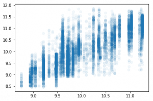
plt.scatter(preds, y_valid, alpha=0.05)
metrics.r2_score(preds, y_valid)

0.4840854669925271
Checking the performance and r-square against the scikit-learn model:
m = RandomForestRegressor(n_estimators=1, min_samples_leaf=5, bootstrap=False)
%time m.fit(x_samp, y_samp)
preds = m.predict(X_valid[cols].values)
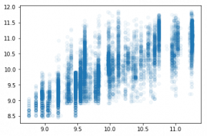
plt.scatter(preds, y_valid, alpha=0.05)
metrics.r2_score(preds, y_valid)

0.47541053100694797
Step 14: Putting it all together!
class TreeEnsemble():
    def __init__(self, x, y, n_trees, sample_sz, min_leaf=5):
        np.random.seed(42)
        self.x,self.y,self.sample_sz,self.min_leaf = x,y,sample_sz,min_leaf
        self.trees = [self.create_tree() for i in range(n_trees)]

    def create_tree(self):
        idxs = np.random.permutation(len(self.y))[:self.sample_sz]
        return DecisionTree(self.x.iloc[idxs], self.y[idxs],
                    idxs=np.array(range(self.sample_sz)), min_leaf=self.min_leaf)

    def predict(self, x):
        return np.mean([t.predict(x) for t in self.trees], axis=0)

def std_agg(cnt, s1, s2): return math.sqrt((s2/cnt) - (s1/cnt)**2)
class DecisionTree():
    def __init__(self, x, y, idxs, min_leaf=5):
        self.x,self.y,self.idxs,self.min_leaf = x,y,idxs,min_leaf
        self.n,self.c = len(idxs), x.shape[1]
        self.val = np.mean(y[idxs])
        self.score = float('inf')
        self.find_varsplit()

    def find_varsplit(self):
        for i in range(self.c): self.find_better_split(i)
        if self.score == float('inf'): return
        x = self.split_col
        lhs = np.nonzero(x<=self.split)[0]
        rhs = np.nonzero(x>self.split)[0]
        self.lhs = DecisionTree(self.x, self.y, self.idxs[lhs])
        self.rhs = DecisionTree(self.x, self.y, self.idxs[rhs])

    def find_better_split(self, var_idx):
        x,y = self.x.values[self.idxs,var_idx], self.y[self.idxs]
        sort_idx = np.argsort(x)
        sort_y,sort_x = y[sort_idx], x[sort_idx]
        rhs_cnt,rhs_sum,rhs_sum2 = self.n, sort_y.sum(), (sort_y**2).sum()
        lhs_cnt,lhs_sum,lhs_sum2 = 0,0.,0.

        for i in range(0,self.n-self.min_leaf):
            xi,yi = sort_x[i],sort_y[i]
            lhs_cnt += 1; rhs_cnt -= 1
            lhs_sum += yi; rhs_sum -= yi
            lhs_sum2 += yi**2; rhs_sum2 -= yi**2
            if i<self.min_leaf-1 or xi==sort_x[i+1]:
                continue

            lhs_std = std_agg(lhs_cnt, lhs_sum, lhs_sum2)
            rhs_std = std_agg(rhs_cnt, rhs_sum, rhs_sum2)
            curr_score = lhs_std*lhs_cnt + rhs_std*rhs_cnt
            if curr_score<self.score:
                self.var_idx,self.score,self.split = var_idx,curr_score,xi

    @property
    def split_name(self): return self.x.columns[self.var_idx]

    @property
    def split_col(self): return self.x.values[self.idxs,self.var_idx]

    @property
    def is_leaf(self): return self.score == float('inf')

    def __repr__(self):
        s = f'n: {self.n}; val:{self.val}'
        if not self.is_leaf:
            s += f'; score:{self.score}; split:{self.split}; var:{self.split_name}'
        return s

    def predict(self, x):
        return np.array([self.predict_row(xi) for xi in x])

    def predict_row(self, xi):
        if self.is_leaf: return self.val
        t = self.lhs if xi[self.var_idx]<=self.split else self.rhs
        return t.predict_row(xi)
ens = TreeEnsemble(X_train[cols], y_train, 5, 1000)
preds = ens.predict(X_valid[cols].values)
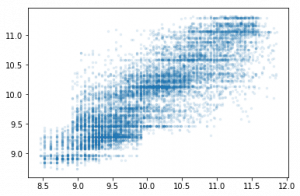
plt.scatter(y_valid, preds, alpha=0.1, s=6);
metrics.r2_score(y_valid, preds)

0.7025757322910476
And there you go! That was quite a learning experience and we have now officially built a machine learning technique right from scratch. Something to be truly proud of!
End Notes
Let’s quickly recap what we covered in part 3. We started with Lesson 6 which broadly covers the applications of machine learning in various business domains and a revision of the interpretation techniques we saw in part 2.
The second half of this article covered Lesson 7 and was a bit code heavy. We built a complete random forest model and compared it’s performance against the scikit-learn’s model. It is a good practice to understand how the model actually works, instead of simply implementing the model.
With this, we come to the end of understanding, interpreting and building a random forest model. In the next part, we will shift our focus to neural networks. We’ll be working on the very popular MNIST dataset so that should be quite fun!


