Introduction
Have you ever been inside a well-maintained library? I’m always incredibly impressed with the way the librarians keep everything organized, by name, content, and other topics. But if you gave these librarians thousands of books and asked them to arrange each book on the basis of their genre, they will struggle to accomplish this task in a day, let alone an hour!
However, this won’t happen to you if these books came in a digital format, right? All the arrangement seems to happen in a matter of seconds, without requiring any manual effort. All hail Natural Language Processing (NLP).

Source: confessionsofabookgeek.com
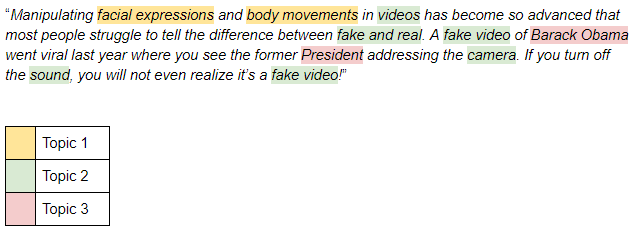
Have a look at the below text snippet:
As you might gather from the highlighted text, there are three topics (or concepts) – Topic 1, Topic 2, and Topic 3. A good topic model will identify similar words and put them under one group or topic. The most dominant topic in the above example is Topic 2, which indicates that this piece of text is primarily about fake videos.
Intrigued, yet? Good! In this article, we will learn about a text mining approach called Topic Modeling. It is an extremely useful technique for extracting topics, and one you will work with a lot when faced with NLP challenges.
Note: I highly recommend going through this article to understand terms like SVD and UMAP. They are leveraged in this article so having a basic understanding of them will help solidify these concepts. We have a paid NLP course as well with a dedicated module for Topic Modeling.
Table of Contents
- What is a Topic Model?
- When is Topic Modeling used?
- Overview of Latent Semantic Analysis (LSA)
- Implementation of LSA in Python
- Data Reading and Inspection
- Data Preprocessing
- Document-Term Matrix
- Topic Modeling
- Topics Visualization
- Pros and Cons of LSA
- Other Techniques for Topic Modeling
What is a topic model?
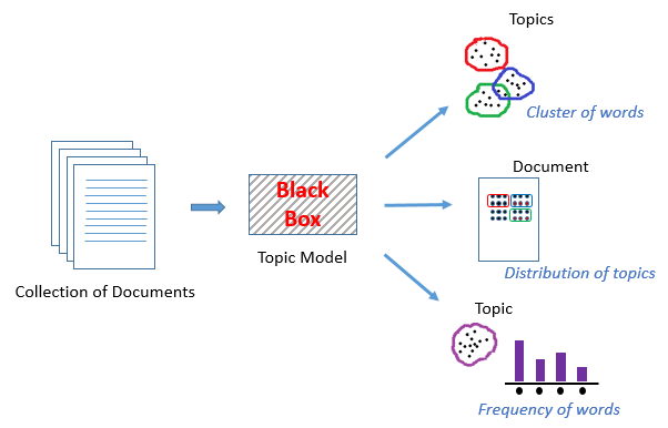
A Topic Model can be defined as an unsupervised technique to discover topics across various text documents. These topics are abstract in nature, i.e., words which are related to each other form a topic. Similarly, there can be multiple topics in an individual document. For the time being, let’s understand a topic model as a black box, as illustrated in the below figure:
This black box (topic model) forms clusters of similar and related words which are called topics. These topics have a certain distribution in a document, and every topic is defined by the proportion of different words it contains.
When is Topic Modeling used?
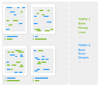
Recall the example we saw earlier of arranging similar books together. Now suppose you have to perform a similar task with a few digital text documents. You would be able to manually accomplish this, as long as the number of documents is manageable (aka not too many of them). But what happens when there’s an impossible number of these digital text documents?
That’s where NLP techniques come to the fore. And for this particular task, topic modeling is the technique we will turn to.
Source: topix.io/tutorial/tutorial.html
Topic modeling helps in exploring large amounts of text data, finding clusters of words, similarity between documents, and discovering abstract topics. As if these reasons weren’t compelling enough, topic modeling is also used in search engines wherein the search string is matched with the results. Getting interesting, isn’t it? Well, read on then!
Overview of Latent Semantic Analysis (LSA)
All languages have their own intricacies and nuances which are quite difficult for a machine to capture (sometimes they’re even misunderstood by us humans!). This can include different words that mean the same thing, and also the words which have the same spelling but different meanings.
For example, consider the following two sentences:
- I liked his last novel quite a lot.
- We would like to go for a novel marketing campaign.
In the first sentence, the word ‘novel’ refers to a book, and in the second sentence it means new or fresh.
We can easily distinguish between these words because we are able to understand the context behind these words. However, a machine would not be able to capture this concept as it cannot understand the context in which the words have been used. This is where Latent Semantic Analysis (LSA) comes into play as it attempts to leverage the context around the words to capture the hidden concepts, also known as topics.
So, simply mapping words to documents won’t really help. What we really need is to figure out the hidden concepts or topics behind the words. LSA is one such technique that can find these hidden topics. Let’s now deep dive into the inner workings of LSA.
Steps involved in the implementation of LSA
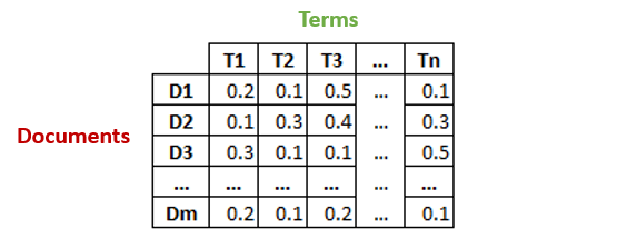
Let’s say we have m number of text documents with n number of total unique terms (words). We wish to extract k topics from all the text data in the documents. The number of topics, k, has to be specified by the user.
- Generate a document-term matrix of shape m x n having TF-IDF scores.
- Then, we will reduce the dimensions of the above matrix to k (no. of desired topics) dimensions, using singular-value decomposition (SVD).
- SVD decomposes a matrix into three other matrices. Suppose we want to decompose a matrix A using SVD. It will be decomposed into matrix U, matrix S, and VT (transpose of matrix V).
Each row of the matrix Uk (document-term matrix) is the vector representation of the corresponding document. The length of these vectors is k, which is the number of desired topics. Vector representation for the terms in our data can be found in the matrix Vk (term-topic matrix).
- So, SVD gives us vectors for every document and term in our data. The length of each vector would be k. We can then use these vectors to find similar words and similar documents using the cosine similarity method.
Implementation of LSA in Python
It’s time to power up Python and understand how to implement LSA in a topic modeling problem. Once your Python environment is open, follow the steps I have mentioned below.
Data reading and inspection
Let’s load the required libraries before proceeding with anything else.
import numpy as np
import pandas as pd
import matplotlib.pyplot as plt
import seaborn as sns
pd.set_option("display.max_colwidth", 200)
In this article, we will use the ’20 Newsgroup’ dataset from sklearn. You can download the dataset here, and follow along with the code.
Python Code:
The dataset has 11,314 text documents distributed across 20 different newsgroups.
Data Preprocessing
To start with, we will try to clean our text data as much as possible. The idea is to remove the punctuations, numbers, and special characters all in one step using the regex replace(“[^a-zA-Z#]”, ” “), which will replace everything, except alphabets with space. Then we will remove shorter words because they usually don’t contain useful information. Finally, we will make all the text lowercase to nullify case sensitivity.
news_df = pd.DataFrame({'document':documents})

# removing everything except alphabets`
news_df['clean_doc'] = news_df['document'].str.replace("[^a-zA-Z#]", " ")

# removing short words
news_df['clean_doc'] = news_df['clean_doc'].apply(lambda x: ' '.join([w for w in x.split() if len(w)>3]))

# make all text lowercase
news_df['clean_doc'] = news_df['clean_doc'].apply(lambda x: x.lower())
It’s good practice to remove the stop-words from the text data as they are mostly clutter and hardly carry any information. Stop-words are terms like ‘it’, ‘they’, ‘am’, ‘been’, ‘about’, ‘because’, ‘while’, etc.
To remove stop-words from the documents, we will have to tokenize the text, i.e., split the string of text into individual tokens or words. We will stitch the tokens back together once we have removed the stop-words.
from nltk.corpus import stopwords
stop_words = stopwords.words('english')

# tokenization
tokenized_doc = news_df['clean_doc'].apply(lambda x: x.split())

# remove stop-words
tokenized_doc = tokenized_doc.apply(lambda x: [item for item in x if item not in stop_words])

# de-tokenization
detokenized_doc = []
for i in range(len(news_df)):
    t = ' '.join(tokenized_doc[i])
    detokenized_doc.append(t)

news_df['clean_doc'] = detokenized_doc
Document-Term Matrix
This is the first step towards topic modeling. We will use sklearn’s TfidfVectorizer to create a document-term matrix with 1,000 terms.
from sklearn.feature_extraction.text import TfidfVectorizer

vectorizer = TfidfVectorizer(stop_words='english',
max_features= 1000, # keep top 1000 terms
max_df = 0.5,
smooth_idf=True)

X = vectorizer.fit_transform(news_df['clean_doc'])

X.shape # check shape of the document-term matrix
(11314, 1000)
We could have used all the terms to create this matrix but that would need quite a lot of computation time and resources. Hence, we have restricted the number of features to 1,000. If you have the computational power, I suggest trying out all the terms.
Topic Modeling
The next step is to represent each and every term and document as a vector. We will use the document-term matrix and decompose it into multiple matrices. We will use sklearn’s TruncatedSVD to perform the task of matrix decomposition.
Since the data comes from 20 different newsgroups, let’s try to have 20 topics for our text data. The number of topics can be specified by using the n_components parameter.
from sklearn.decomposition import TruncatedSVD

# SVD represent documents and terms in vectors
svd_model = TruncatedSVD(n_components=20, algorithm='randomized', n_iter=100, random_state=122)

svd_model.fit(X)

len(svd_model.components_)
20
The components of svd_model are our topics, and we can access them using svd_model.components_. Finally, let’s print a few most important words in each of the 20 topics and see how our model has done.
terms = vectorizer.get_feature_names()

for i, comp in enumerate(svd_model.components_):
    terms_comp = zip(terms, comp)
    sorted_terms = sorted(terms_comp, key= lambda x:x[1], reverse=True)[:7]
    print("Topic "+str(i)+": ")
    for t in sorted_terms:
        print(t[0])
        print(" ")
Topic 0: like know people think good time thanks
Topic 1: thanks windows card drive mail file advance
Topic 2: game team year games season players good
Topic 3: drive scsi disk hard card drives problem
Topic 4: windows file window files program using problem
Topic 5: government chip mail space information encryption data
Topic 6: like bike know chip sounds looks look
Topic 7: card sale video offer monitor price jesus
Topic 8: know card chip video government people clipper
Topic 9: good know time bike jesus problem work
Topic 10: think chip good thanks clipper need encryption
Topic 11: thanks right problem good bike time window
Topic 12: good people windows know file sale files
Topic 13: space think know nasa problem year israel
Topic 14: space good card people time nasa thanks
Topic 15: people problem window time game want bike
Topic 16: time bike right windows file need really
Topic 17: time problem file think israel long mail
Topic 18: file need card files problem right good
Topic 19: problem file thanks used space chip sale
Topics Visualization
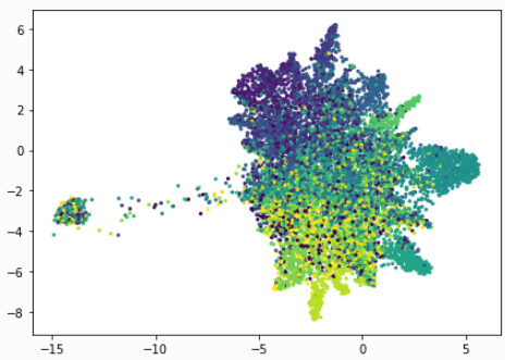
To find out how distinct our topics are, we should visualize them. Of course, we cannot visualize more than 3 dimensions, but there are techniques like PCA and t-SNE which can help us visualize high dimensional data into lower dimensions. Here we will use a relatively new technique called UMAP (Uniform Manifold Approximation and Projection).
import umap

X_topics = svd_model.fit_transform(X)
embedding = umap.UMAP(n_neighbors=150, min_dist=0.5, random_state=12).fit_transform(X_topics)

plt.figure(figsize=(7,5))
plt.scatter(embedding[:, 0], embedding[:, 1],
c = dataset.target,
s = 10, # size
edgecolor='none'
)
plt.show()
As you can see above, the result is quite beautiful. Each dot represents a document and the colours represent the 20 newsgroups. Our LSA model seems to have done a good job. Feel free to play around with the parameters of UMAP to see how the plot changes its shape.
The entire code for this article can be found in this GitHub repository.
Pros and Cons of LSA
Latent Semantic Analysis can be very useful as we saw above, but it does have its limitations. It’s important to understand both the sides of LSA so you have an idea of when to leverage it and when to try something else.
Pros:
- LSA is fast and easy to implement.
- It gives decent results, much better than a plain vector space model.
Cons:
- Since it is a linear model, it might not do well on datasets with non-linear dependencies.
- LSA assumes a Gaussian distribution of the terms in the documents, which may not be true for all problems.
- LSA involves SVD, which is computationally intensive and hard to update as new data comes up.
Other Techniques for Topic Modeling
Apart from LSA, there are other advanced and efficient topic modeling techniques such as Latent Dirichlet Allocation (LDA) and lda2Vec. We have a wonderful article on LDA which you can check out here. lda2vec is a much more advanced topic modeling which is based on word2vec word embeddings. If you want to find out more about it, let me know in the comments section below and I’ll be happy to answer your questions/.
End Notes
This article is an attempt to share my learnings with all of you. Topic modeling is quite an interesting topic and equips you with the skills and techniques to work with many text datasets. So, I urge you all to use the code given in this article and apply it to a different dataset. Let me know if you have any questions or feedback related to this article. Happy text mining!



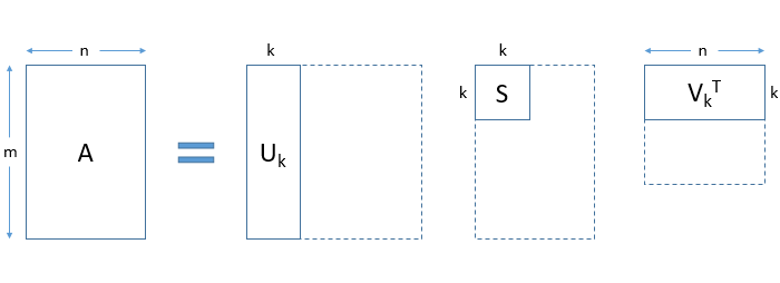 Each row of the matrix Uk (document-term matrix) is the vector representation of the corresponding document. The length of these vectors is k, which is the number of desired topics. Vector representation for the terms in our data can be found in the matrix Vk (term-topic matrix).