Introduction
The human heart, a complex and vital organ, has been the subject of countless studies, breakthroughs, and innovations in the field of medical research. One such innovation is echocardiography, a non-invasive imaging technique that has revolutionized how we visualize and assess heart function. With the advent of advanced machine learning algorithms, extracting crucial information from these images has become an area of active research. In this blog post, we will delve into the world of biomedical image segmentation, focusing on the left ventricle of the heart, an essential component of our circulatory system. Join me as I preprocess the Cardiac Acquisitions for Multi-structure Ultrasound Segmentation (CAMUS) dataset, walking you through each step in Python to ensure your segmentation model has a strong foundation to build upon.
A Complete Python Tutorial to Learn Data Science from Scratch
Learning Objective:
Explore the process of preprocessing the Cardiac Acquisitions for the Multi-structure Ultrasound Segmentation (CAMUS) dataset. The creators designed the CAMUS dataset for evaluating left ventricle segmentation and ejection fraction assessment algorithms in echocardiography, and it is publicly available. It consists of 2D echocardiographic images acquired from different views, such as the four-chamber (4ch) view. Preprocessing is essential in building an accurate segmentation model. It improves the quality of input data and ensures that the model is trained on consistent and normalized data. This tutorial will use Python and various libraries to preprocess the images and their corresponding masks.

This article was published as a part of the Data Science Blogathon.
Table of Contents
Dataset Overview
The Cardiac Acquisitions for Multi-structure Ultrasound Segmentation dataset can be downloaded from the following link: https://www.creatis.insa-lyon.fr/Challenge/camus/. It contains 500 image sequences with corresponding expert-drawn contours of the left ventricle. This tutorial will focus on the 4ch view images and masks. The images are provided in MetaImage (.mhd) format, which requires specialized libraries like SimpleITK for reading and processing.
Preprocessing Steps
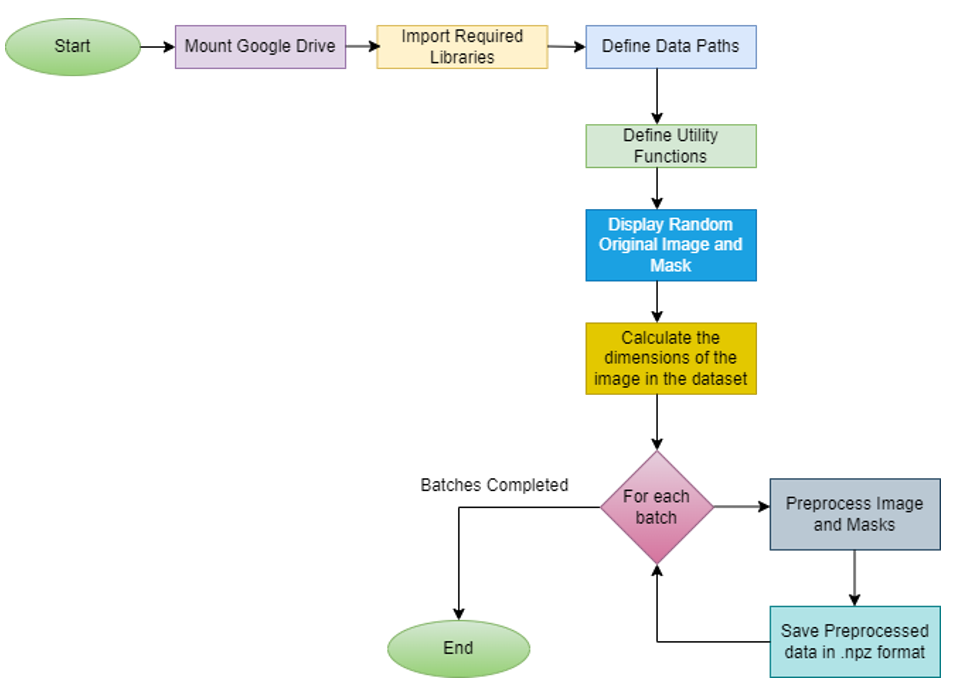
- Mount Google Drive to access the dataset.
- Install required libraries (SimpleITK, h5py).
- Set dataset paths.
- Define helper functions for data normalization, reading image data, and resizing.
- Visualize random images and masks from the dataset.
- Calculate image dimensions (width and length).
- Resize images and masks to consistent dimensions.
- Normalize image pixel values.
- Save preprocessed images and masks in batches.
Here is an overview of the steps in the form of a flowchart for the preprocessing of CAMUS image datasets:
Code Walkthrough
First, we mount Google Drive to access the dataset and install the required libraries (SimpleITK, h5py) using the !pip install command.
Mount Google Drive to access the dataset
from google.colab import drive
drive.mount('/content/drive')
The code from Google.colab import drive is importing the necessary module drive from Google.colab
package. This package provides tools for working with Google Colaboratory, a free cloud-based coding, and data analysis platform.
The next line drive.mount(‘/content/drive’) calls the mount() function from the drive module to mount your Google Drive account. This allows you to access files and folders stored in your Google Drive directly from your Colab notebook.
Running this code will prompt you to authorize access to your Google Drive account by following a URL and entering an authorization code. Once this step is complete, your Google Drive will be mounted, and you will be able to access files in your Drive using the file path /content/drive/ within your Colab notebook.
Overall, this code is setting up the necessary configuration to enable you to access files in your Google Drive within the Colab environment, which can be useful for working with data or files that you have stored in the cloud.
Install Required lLibraries(SimpleITK, h5py)
import os
import numpy as np
import pandas as pd
import time
import random
from contextlib import contextmanager
from functools import partial
import seaborn as sns
import SimpleITK as sitk
import matplotlib.pylab as plt
%matplotlib inline
import cv2
from tqdm.notebook import tqdm
import h5py
from skimage.transform import resize

!pip install SimpleITK
!pip install h5py
The first few lines of the code are importing necessary Python modules like os, numpy, pandas, time, random, contextlib, functools, seaborn, SimpleITK, matplotlib, cv2, tqdm, and h5py. These modules provide functions and classes for working with arrays, dataframes, plotting, image processing, and more.
The next two lines install the SimpleITK and h5py libraries using pip, which allows you to use these libraries in your code.
Overall, this code imports necessary Python modules, set up paths to data directories and defines helper functions for measuring the time a code block takes. It is setting up the necessary configuration for working with data for a cardiac image analysis task.
Set Dataset Paths.
data_path = "/content/drive/MyDrive/CAM/LVEF/CAMUS/original_data/data/training/4ch/"

if os.path.exists(data_path):
    print(f"Path exists: {data_path}")
else:
    print(f"Path not found: {data_path}")

fig_size = plt.rcParams["figure.figsize"]
fig_size[0] = 7
fig_size[1] = 9
plt.rcParams["figure.figsize"] = fig_size

@contextmanager
def timer(name):
    t0 = time.time()
    yield
    print(f'[{name}] done in {time.time() - t0:.0f} s')

ROOT_PATH='/content/drive/MyDrive/CAM/LVEF/CAMUS/original_data/data/'
TRAIN_PATH=ROOT_PATH+'training/'
TEST_PATH=ROOT_PATH+'testing/'
The next block of code sets the data_path variable to the location of the training data for a cardiac image analysis task. It checks whether the specified path exists using the os.path.exists() function and prints a
a message to the console indicating whether the path was found or not.
The next block of code sets the size of the plot figure using plt.rcParams[“figure.figsize”] and sets up a timer function using a context manager. The timer function is used to measure the time taken to run a code block.
Finally, the code sets up several variables with paths to different directories within the original data folder, which is located in a Google Drive account (ROOT_PATH, TRAIN_PATH, and TEST_PATH). These variables will be used later in the code to load and process data for the cardiac image analysis task.
Define Helper Functions for Data Normalization, Reading Image Data, and Resizing
def data_norm(input):
    input = np.array(input, dtype=np.float32)
    input  = input - np.mean(input)
    output = input / (np.std(input) + 1e-12)
    return output

def mhd_to_array(path):
    return sitk.GetArrayFromImage(sitk.ReadImage(path, sitk.sitkFloat32))

def read_info(data_file):
  info = {}
  with open(data_file, 'r') as f:
    for line in f.readlines():
      info_type, info_details = line.strip('\n').split(': ')
      info[info_type] = info_details
  return info

def plot_histogram(image, title):
    plt.figure()
    plt.hist(image.ravel(), bins=256)
    plt.title(title)
    plt.xlabel('Pixel Intensity')
    plt.ylabel('Frequency')
    plt.show()

def plot_random_image_and_mask(image_folder, mask_folder, image_files, mask_files):
    index = random.randint(0, len(image_files) - 1)

    img_path = os.path.join(image_folder, image_files[index])
    mask_path = os.path.join(mask_folder, mask_files[index])

    img = sitk.GetArrayFromImage(sitk.ReadImage(img_path, sitk.sitkFloat32))
    mask = sitk.GetArrayFromImage(sitk.ReadImage(mask_path, sitk.sitkFloat32))

    fig, ax = plt.subplots(1, 2, figsize=(10, 10))
    ax[0].imshow(img[0], cmap='gray')
    ax[0].axis('off')
    ax[0].set_title('Image')
    ax[1].imshow(mask[0], cmap='gray')
    ax[1].axis('off')
    ax[1].set_title('Mask')
    plt.show()
This code defines several functions for image processing and visualization:
- data_norm(input): This function takes an input image as an array, normalizes it by subtracting the mean and dividing by the standard deviation, and returns the normalized image.
- mhd_to_array(path): This function reads a .mhd image file from the specified path using SimpleITK and returns the image as a NumPy array.
- read_info(data_file): This function reads information about the image from the specified file and returns it as a dictionary.
- plot_histogram(image, title): This function plots a histogram of pixel intensities for the specified image with the given title.
- plot_random_image_and_mask(image_folder, mask_folder, image_files, mask_files): This function selects a random image and mask from the specified folders and files, reads them using SimpleITK, and displays them side-by-side in a plot.
These functions are likely being used in a larger image processing or machine learning project to preprocess and visualize medical image data.
Visualize Random Images and Masks From the Dataset
image_files = sorted([f for f in os.listdir(TRAIN_PATH + "4ch/frames") if f.endswith('.mhd')])
mask_files = sorted([f for f in os.listdir(TRAIN_PATH + "4ch/masks") if f.endswith('.mhd')])

plot_random_image_and_mask(TRAIN_PATH + "4ch/frames", TRAIN_PATH + "4ch/masks", image_files, mask_files)#import csv
This code block creates two lists, image_files, and mask_files, containing the names of all .mhd files in the training set for the 4ch (four chambers) view of the heart. The sorted function is used to sort the file names in ascending order.
Then, the plot_random_image_and_mask function is called with the paths to the image and mask folders (TRAIN_PATH + “4ch/frames” and TRAIN_PATH + “4ch/masks”, respectively) and the lists of file names as arguments (image_files and mask_files). This function selects a random image and mask from the specified folders using the random module, reads them using SimpleITK, and displays them side-by-side in a plot using Matplotlib.
The purpose of this code block is likely to visualize a random image and corresponding mask from the training set for the 4ch view, which can help to verify that the data is being read and processed correctly.
Calculate Image Dimensions (Width and Length)
widths = []
lengths = []
clst=['4ch']
for c in clst:
    file_list = os.listdir(os.path.join(TRAIN_PATH, c+"/frames"))
    for i in file_list:
        if "mhd" in i:
            path=TRAIN_PATH+c+"/frames/"+ i
            w = mhd_to_array(path).shape[2]
            l = mhd_to_array(path).shape[1]
            widths.append(w)
            lengths.append(l)
print('Max width : ',max(widths))
print('Min width : ',min(widths))
print('Max length : ',max(lengths))
print('Min length : ',min(lengths))
This code computes the images’ maximum and minimum width and length in the specified directory.
The list of folders to be considered is contained in the variable clst. In this case, it only contains “4ch”.
The code then iterates through all the files in the specified directory for each folder in clst, and checks if the file has the extension “.mhd.” If so, it reads the file using the mhd_to_array() function and retrieves its width and length using the .shape[2] and .shape[1] attributes, respectively. We then append the width and length to the list’s widths and lengths.
Finally, we print the maximum and minimum values of the widths and lengths lists using the max() and min() functions.
Resize Images and Masks to Consistent Dimensions
def resize_image(image, width, height):
    return resize(image, (height, width), preserve_range=True, mode='reflect', anti_aliasing=True)

def preprocess_images_and_masks(image_folder, mask_folder, width, height, image_files, mask_files):
    preprocessed_images = []
    preprocessed_masks = []

    for img_file, mask_file in tqdm(zip(image_files, mask_files), total=len(image_files)):
        img_path = os.path.join(image_folder, img_file)
        mask_path = os.path.join(mask_folder, mask_file)

        img = mhd_to_array(img_path)
        mask = mhd_to_array(mask_path)

        img_resized = np.zeros((img.shape[0], height, width), dtype=np.float32)
        mask_resized = np.zeros((mask.shape[0], height, width), dtype=np.float32)

        for i in range(img.shape[0]):
            img_resized[i] = resize_image(img[i], width, height)
            mask_resized[i] = resize_image(mask[i], width, height)

        img_normalized = data_norm(img_resized)

        preprocessed_images.append(img_normalized)
        preprocessed_masks.append(mask_resized)

    return preprocessed_images, preprocessed_masks
This code defines a function called resize_image that resizes an image to a specified width and height using the resize function from the skimage library. You can pass three arguments to the function: the image you want to resize, the desired width, and the desired height. We set the preserve_range argument to True to ensure that the pixel values of the resized image are within the same range as the original image. We set the mode argument to ‘reflect’ to handle the edges of the image, and we set anti_aliasing to True to smooth out the image.
The preprocess_images_and_masks function takes in a folder containing images and a folder containing
corresponding masks, as well as the desired width and height for resizing. It also takes in lists of image and mask files. The function then loops through each pair of image and mask files. It also reads in the images and masks using the mhd_to_array function, resizes the images and masks using the resize_image function, and normalizes the resized images using the data_norm function defined earlier. The function appends the preprocessed images and masks to two separate lists and then returns them.
Normalize Image Pixel Values
RESIZED_WIDTH = 256
RESIZED_LENGTH = 256
BATCH_SIZE = 8

image_files = sorted([f for f in os.listdir(TRAIN_PATH + "4ch/frames") if f.endswith('.mhd')])
mask_files = sorted([f for f in os.listdir(TRAIN_PATH + "4ch/masks") if f.endswith('.mhd')])

preprocessed_data_path = "/content/drive/MyDrive/CAM/CAM1/preprocessed_data/"

if not os.path.exists(preprocessed_data_path):
    os.makedirs(preprocessed_data_path)

for batch_start in range(0, len(image_files), BATCH_SIZE):
    batch_end = min(batch_start + BATCH_SIZE, len(image_files))
    X_batch, y_batch = preprocess_images_and_masks(
        TRAIN_PATH + "4ch/frames", TRAIN_PATH + "4ch/masks",
        RESIZED_WIDTH, RESIZED_LENGTH,
        image_files[batch_start:batch_end], mask_files[batch_start:batch_end]
    )
This code preprocesses the images and masks for a deep learning model by resizing them to a fixed size and normalizing the pixel values.
The RESIZED_WIDTH and RESIZED_LENGTH variables define the width and height of the resized images, respectively. The BATCH_SIZE variable determines how many images are processed at a time.
The image_files and mask_files variables are lists of file names of the input images and masks, respectively. We use the sorted function to ensure that the images and masks are in the same order.
If the directory specified in the preprocessed_data_path variable does not exist, the function creates it using os.makedirs. We will save the preprocessed data here.
The for loop iterates over the input images and masks in batches of size BATCH_SIZE. Each batch’s preprocess_images_and_masks function is called to resize and normalize the images and masks.
Save Preprocessed Images and Masks in Batches
np.savez(
        preprocessed_data_path + f"preprocessed_data_batch_{batch_start}_{batch_end}.npz",
        X=X_batch, y=y_batch
    )
We can save the resulting preprocessed data to a NumPy archive file using np.savez. The file name of each archive file includes the batch start and end indices. Keeping track of which images and masks are processed in that batch is helpful.
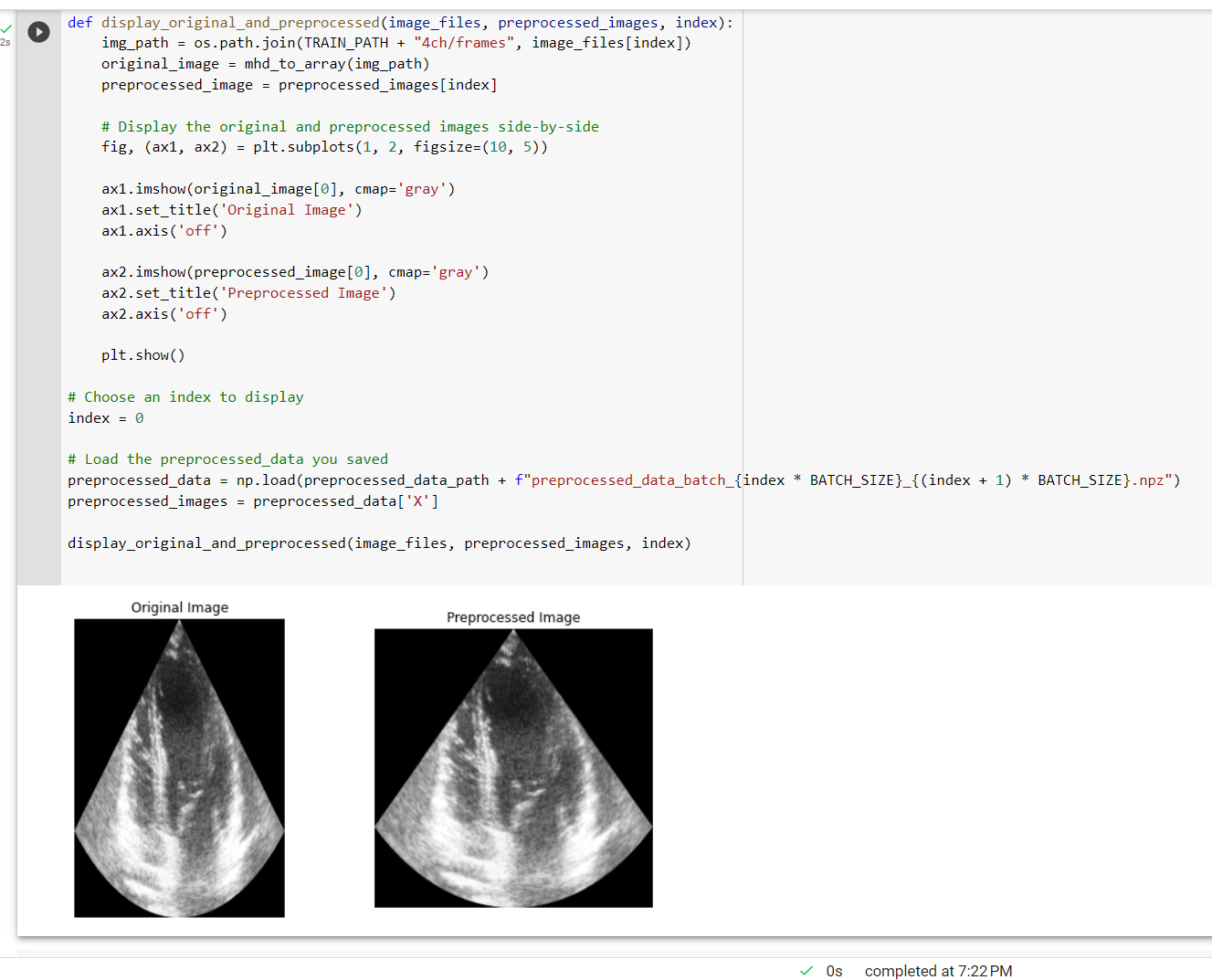
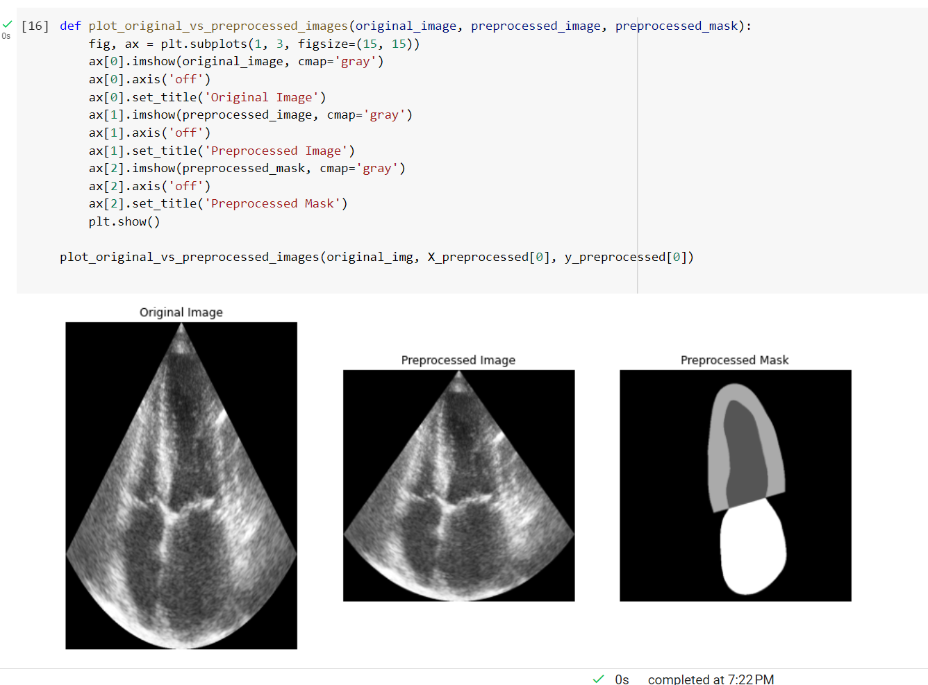
In the world of medical image analysis, preprocessing plays a pivotal role in enhancing the quality and interpretability of the images. This helps improves the understanding of human experts. Additionally, it also significantly boosts the performance of ML algorithms. Let’s now dive deep into the power of preprocessing. We will do this by examining its impact on the Cardiac Acquisitions for the Multi-structure Ultrasound Segmentation dataset. Get ready to witness a striking transformation! I will unveil a side-by-side comparison of the original and preprocessed images, showcasing the remarkable improvements achieved through our preprocessing pipeline.
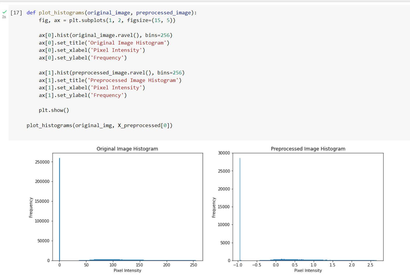
Embark on a captivating exploration of the world of image histograms. Here we will unravel the subtle nuances between original and preprocessed medical images. Here is a stunning visual comparison of histograms that vividly highlight the impact of preprocessing on the Cardiac Acquisitions for the Multi-structure Ultrasound Segmentation dataset. Witness the fascinating transformation as we delve into the realm of pixel intensity distributions. We will also shed light on the remarkable enhancements achieved through our preprocessing techniques.
Finally, in our latest blog post, let’s witness an interplay between original, preprocessed images and their corresponding masks.
Aspects To Consider
Here are some important aspects to consider when working with Cardiac Acquisitions for Multi-structure Ultrasound Segmentation datasets and image segmentation in general:
- Data Augmentation: We can use data augmentation as a technique to increase the amount of training data. It involves applying various transformations to the existing dataset. This helps in improving the generalization capabilities of a model. For echocardiographic images, you can use techniques such as rotation, scaling, flipping, and brightness/contrast adjustments. Make sure to apply the same transformations to both the images and their corresponding masks.
- Train-Validation Split: Divide your dataset into training and validation. This help sets to monitor the model’s performance during training and prevent overfitting. A typical ratio is 80% for training and 20% for validation. Ensure that you perform the split randomly and in a stratified manner, where the distribution of classes is similar in both sets.
- Choice of Model Architecture: The choice of the model architecture plays a significant role in the performance of the segmentation task. U-Net is a popular convolutional neural network architecture for biomedical image segmentation. Various applications have demonstrated its effectiveness of it. We can also consider other architectures like DeepLabv3 and Mask R-CNN for segmentation tasks.
- Loss Functions: The choice of the loss function is crucial for training a segmentation model. Commonly used loss functions for segmentation tasks are Dice loss, Jaccard/Intersection over Union (IoU) loss, and Binary Cross-Entropy loss. You can also experiment with a combination of these loss functions to achieve better performance.
- Evaluation Metrics: Use appropriate evaluation metrics to measure the performance of your segmentation model. Common metrics for segmentation tasks are the Dice coefficient, Jaccard/Intersection over Union (IoU) score, sensitivity, specificity, and accuracy. Track these metrics during training to ensure that your model learns the desired patterns from the data.
- Post-Processing: We can apply post-processing techniques to improve the final results of the segmentation model on its output. Some common post-processing techniques include morphological operations (e.g., dilation, erosion), hole filling, and contour smoothing. These techniques can help refine the segmentation output and produce better contours.
Conclusion
In conclusion, this blog discussed the importance of preprocessing the CAMUS dataset for efficient utilization in cardiovascular imaging analysis. Researchers and practitioners can optimize the dataset by applying various preprocessing techniques. This can help develop and test models in the medical imaging
field.
Key takeaways:
- Preprocessing the CAMUS dataset is crucial for effective use in cardiovascular imaging analysis.
- Techniques such as image resizing, normalization, and data augmentation can improve the dataset’s usability.
- Preprocessed data helps researchers and practitioners develop and test more accurate and efficient models in medical imaging.
Follow me to stay updated on the next steps for achieving promising results in LV segmentation and performance metrics visualizations.
The media shown in this article is not owned by Analytics Vidhya and is used at the Author’s discretion.


