Introduction
The best way to learn data science is to do data science. No second thought about it!
One of the ways, I do this is continuously look for interesting work done by other community members. Once I understand the project, I do / improve the project on my own. Honestly, I can’t think of a better way to learn data science.
As part of my search, I came across a study on sentiment analysis of Chennai Floods on Analytics Vidhya. I decided to perform sentiment analysis of the same study using Python and add it here. Well, what can be better than building onto something great.
To get acquainted with the crisis of Chennai Floods, 2015 you can read the complete study here. This study was done on a set of social interactions limited to the first two days of Chennai Floods in December 2015.
The objectives of this article is to understand the different subjects of interactions during the floods using Python. Grouping similar messages together with emphasis on predominant themes (rescue, food, supplies, ambulance calls) can help government and other authorities to act in the right manner during the crisis time.
Building Corpus
A typical tweet is mostly a text message within limit of 140 characters. #hashtags convey subject of the tweet whereas @user seeks attention of that user. Forwarding is denoted by ‘rt’ (retweet) and is a measure of its popularity. One can like a tweet by making it ‘favorite’.
About 6000 twits were collected with ‘#ChennaiFloods’ hashtag and between 1st and 2nd Dec 2015. Jefferson’s GetOldTweets utility (got) was used in Python 2.7 to collect the older tweets. One can store the tweets either in a csv file or to a database like MongoDb to be used for further processing.
import got, codecsfrom pymongo import MongoClientclient = MongoClient('localhost', 27017)db = client['twitter_db']collection = db['twitter_collection']tweetCriteria =got.manager.TweetCriteria().setQuerySearch('ChennaiFloods').setSince("2015-12-01").setUntil("2015-12-02").setMaxTweets(6000)def streamTweets(tweets):for t in tweets:obj = {"user": t.username, "retweets": t.retweets, "favorites": t.favorites, "text":t.text,"geo": t.geo,"mentions": t.mentions, "hashtags": t.hashtags,"id": t.id, "permalink": t.permalink,}tweetind = collection.insert_one(obj).inserted_idgot.manager.TweetManager.getTweets(tweetCriteria, streamTweets)
Tweets stored in MongoDB can be accessed from another python script. Following example shows how the whole db was converted to Pandas dataframe.
import pandas as pdfrom pymongo import MongoClient client = MongoClient ('localhost', 27017) db = client ['twitter_db'] collection = db ['twitter_collection'] df=pd.DataFrame(list(collection.find()))
First few records of the dataframe look as below:
Data Exploration
Once in dataframe format, it is easier to explore the data. Here are few examples:
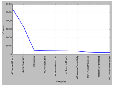
hashtags = []for hs in df["hashtags"]: # Each entry may contain multiple hashtags. Split.hashtags += hs.split(" ")fdist1 = FreqDist(hashtags)fdist1.plot(10)

Top 10 Hashtags trending
As seen in the study the most used tags were “#chennairains”, “#ICanAccommodate”, apart from the original query tag “#ChennaiFloods”.
- Top 10 users
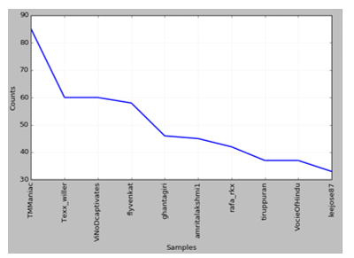
users = df["user"].tolist()fdist2 = FreqDist(users)fdist2.plot(10)
As seen from the plot, most active users were “TMManiac” with about 85 tweets, “Texx_willer” with 60 tweets and so on…

Top 10 Users tweeting
Text Pre-processing
All tweets are processed to remove unnecessary things like links, non-English words, stopwords, punctuation’s, etc.
from nltk.tokenize import TweetTokenizerfrom nltk.corpus import stopwordsimport re, stringimport nltktweets_texts = df["text"].tolist()stopwords=stopwords.words('english')english_vocab = set(w.lower() for w in nltk.corpus.words.words())def process_tweet_text(tweet):if tweet.startswith('@null'):return "[Tweet not available]" tweet = re.sub(r'\$\w*','',tweet) # Remove tickers tweet = re.sub(r'https?:\/\/.*\/\w*','',tweet) # Remove hyperlinks tweet = re.sub(r'['+string.punctuation+']+', ' ',tweet) # Remove puncutations like 's twtok = TweetTokenizer(strip_handles=True, reduce_len=True)tokens = twtok.tokenize(tweet)tokens = [i.lower() for i in tokens if i not in stopwords and len(i) > 2 and i in english_vocab]return tokenswords = []for tw in tweets_texts:words += process_tweet_text(tw)
The word list generated looks like:
[‘time’, ‘history’, ‘temple’, ‘closed’, ‘due’, ‘pic’, ‘twitter’, ‘havoc’, ‘incessant’, …]
Text Exploration
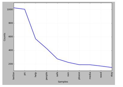
The words are plotted again to find the most frequently used terms. A few simple words repeat more often than others: ’help’, ‘people’, ‘stay’, ’safe’, etc.
[(‘twitter’, 1026), (‘pic’, 1005), (‘help’, 569), (‘people’, 429), (‘safe’, 274)]
These are immediate reactions and responses to the crisis.
Some infrequent terms are [(‘fit’, 1), (‘bible’, 1), (‘disappear’, 1), (‘regulated’, 1), (‘doom’, 1)].

Most frequently used words
Collocations are the words that are found together. They can be bi-grams (two words together) or phrases like trigrams (3 words) or n-grams (n words).
from nltk.collocations import *
bigram_measures = nltk.collocations.BigramAssocMeasures()
finder = BigramCollocationFinder.from_words(words, 5)
finder.apply_freq_filter(5)
print(finder.nbest(bigram_measures.likelihood_ratio, 10))
Most frequently appearing Bigrams are:
[(‘pic’, ‘twitter’), (‘lady’, ‘labour’), (‘national’, ‘media’), (‘pani’, ‘pani’), (‘team’, ‘along’), (‘stay’, ‘safe’), (‘rescue’, ‘team’), (‘beyond’, ‘along’), (‘team’, ‘beyond’), (‘rescue’, ‘along’)]
These depict the disastrous situation, like “stay safe”, “rescue team”, even a commonly used Hindi phrase “pani pani” (lots of water).
Clustering
In such crisis situations, lots of similar tweets are generated. They can be grouped together in clusters based on closeness or ‘distance’ amongst them. Artem Lukanin has explained the process in details here. TF-IDF method is used to vectorize the tweets and then cosine distance is measured to assess the similarity.
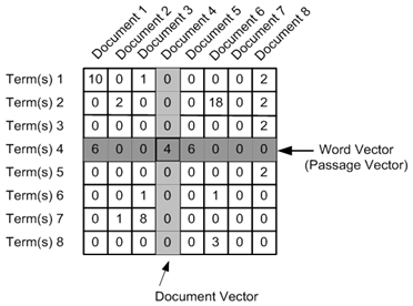
Each tweet is pre-processed and added to a list. The list is fed to TFIDF Vectorizer to convert each tweet into a vector. Each value in the vector depends on how many times a word or a term appears in the tweet (TF) and on how rare it is amongst all tweets/documents (IDF). Below is a visual representation of TFIDF matrix it generates.
Before using the Vectorizer, the pre-processed tweets are added in the data frame so that each tweets association with other parameters like id, user is maintained.
cleaned_tweets = []for tw in tweets_texts:words = process_tweet_text(tw)cleaned_tweet = " ".join(w for w in words if len(w) > 2 andw.isalpha()) #Form sentences of processed wordscleaned_tweets.append(cleaned_tweet)df['CleanTweetText'] = cleaned_tweets
Vectorization is done using 1-3 n-grams, meaning phrases with 1,2,3 words are used to compute frequencies, i.e. TF IDF values. One can get cosine similarity amongst tweets/documents as well.
from sklearn.feature_extraction.text import TfidfVectorizertfidf_vectorizer = TfidfVectorizer(use_idf=True, ngram_range=(1,3))tfidf_matrix = tfidf_vectorizer.fit_transform(cleaned_tweets)feature_names = tfidf_vectorizer.get_feature_names() # num phrasesfrom sklearn.metrics.pairwise import cosine_similaritydist = 1 - cosine_similarity(tfidf_matrix)print(dist)from sklearn.cluster import KMeansnum_clusters = 3km = KMeans(n_clusters=num_clusters)km.fit(tfidf_matrix)clusters = km.labels_.tolist()df['ClusterID'] = clustersprint(df['ClusterID'].value_counts())
K-means clustering algorithm is used to group tweets into choosen number (say, 3) of groups.
The output shows 3 clusters, with following number of tweets in respective clusters.
Most of the tweets are clustered around in group Id =1. Remaining are in group id 2 and id 0.
The top words used in each cluster can be computed by as follows:
#sort cluster centers by proximity to centroid order_centroids = km.cluster_centers_.argsort()[:, ::-1]for i in range(num_clusters):print("Cluster {} : Words :".format(i))for ind in order_centroids[i, :10]:print(' %s' % feature_names[ind])
The result is:
- Cluster 0: Words: show mercy please people rain
- Cluster 1: Words: pic twitter zoo wall broke ground saving guilty water growing
- Cluster 2: Words: help people pic twitter safe open rain share please
Topic Modeling
Finding central subject in the set of documents, tweets in case here. Following are two ways of detecting topics, i.e. clustering the tweets
Latent Dirichlet Allocation (LDA)
LDA is commonly used to identify chosen number (say, 6) topics. Refer tutorial for more details.
from gensim import corpora, modelsfrom nltk.corpus import stopwordsfrom nltk.stem.wordnet import WordNetLemmatizerimport stringstop = set(stopwords.words('english'))exclude = set(string.punctuation)lemma = WordNetLemmatizer()def clean(doc):stop_free = " ".join([i for i in doc.lower().split() if i not in stop])punc_free = ''.join(ch for ch in stop_free if ch not in exclude)normalized = " ".join(lemma.lemmatize(word) for word in punc_free.split())return normalizedtexts = [text for text in cleaned_tweets if len(text) > 2]doc_clean = [clean(doc).split() for doc in texts]dictionary = corpora.Dictionary(doc_clean)doc_term_matrix = [dictionary.doc2bow(doc) for doc in doc_clean]ldamodel = models.ldamodel.LdaModel(doc_term_matrix, num_topics=6, id2word = dictionary, passes=5)for topic in ldamodel.show_topics(num_topics=6, formatted=False, num_words=6):print("Topic {}: Words: ".format(topic[0]))topicwords = [w for (w, val) in topic[1]]print(topicwords)
The output gives us following set of words for each topic.
It is clear from the words associated with the topics that they represent certain sentiments. Topic 0 is about Caution, Topic 1 is about Help, Topic 2 is about News, etc.
Doc2Vec and K-means
Doc2Vec methodology available in gensim package is used to vectorize the tweets, as follows:
import gensimfrom gensim.models.doc2vec import TaggedDocumenttaggeddocs = []tag2tweetmap = {}for index,i in enumerate(cleaned_tweets):if len(i) > 2: # Non empty tweets tag = u'SENT_{:d}'.format(index)sentence = TaggedDocument(words=gensim.utils.to_unicode(i).split(), tags=[tag])tag2tweetmap[tag] = itaggeddocs.append(sentence) model = gensim.models.Doc2Vec(taggeddocs, dm=0, alpha=0.025, size=20, min_alpha=0.025, min_count=0)for epoch in range(60):if epoch % 20 == 0:print('Now training epoch %s' % epoch)model.train(taggeddocs)model.alpha -= 0.002 # decrease the learning rate model.min_alpha = model.alpha # fix the learning rate, no decay
Once trained model is ready the tweet-vectors available in model can be clustered using K-means.
from sklearn.cluster import KMeansdataSet = model.syn0kmeansClustering = KMeans(n_clusters=6)centroidIndx = kmeansClustering.fit_predict(dataSet)topic2wordsmap = {}for i, val in enumerate(dataSet):tag = model.docvecs.index_to_doctag(i)topic = centroidIndx[i]if topic in topic2wordsmap.keys():for w in (tag2tweetmap[tag].split()):topic2wordsmap[topic].append(w)else:topic2wordsmap[topic] = []for i in topic2wordsmap:words = topic2wordsmap[i]print("Topic {} has words {}".format(i, words[:5]))
The result is the list of topics and commonly used words in each, respectively.
It is clear from the words associated with the topics that they represent certain sentiments. Topic 0 is about Caution, Topic 1 is about Actions, Topic 2 is about Climate, etc.The result is the list of topics and commonly used words in each, respectively.
End Notes
This article shows how to implement Capstone-Chennai Floods study using Python and its libraries. With this tutorial, one can get introduction to various Natural Language Processing (NLP) workflows such as accessing twitter data, pre-processing text, explorations, clustering and topic modeling.


