Overview
- Free tutorial to learn Data Science in R for beginners
- Covers predictive modeling, data manipulation, data exploration, and machine learning algorithms in R
Introduction
R is a powerful language used widely for data analysis and statistical computing. It was developed in early 90s. Since then, endless efforts have been made to improve R’s user interface. The journey of R language from a rudimentary text editor to interactive R Studio and more recently Jupyter Notebooks has engaged many data science communities across the world.
This was possible only because of generous contributions by R users globally. Inclusion of powerful packages in R has made it more and more powerful with time. Packages such as dplyr, tidyr, readr, data.table, SparkR, ggplot2 have made data manipulation, visualization and computation much faster.
But, what about Machine Learning?
My first impression of R was that it’s just a software for statistical computing. Good thing, I was wrong! R has enough provisions to implement machine learning algorithms in a fast and simple manner.
This is a complete tutorial to learn data science and machine learning using R. By the end of this tutorial, you will have a good exposure to building predictive models using machine learning on your own.
Note: No prior knowledge of data science / analytics is required. However, prior knowledge of algebra and statistics will be helpful.

A Complete Tutorial to learn Data Science in R from Scratch
Table of Contents
- Basics of R Programming for Data Science
- Why learn R ?
- How to install R / R Studio ?
- How to install R packages ?
- Basic computations in R
- Essentials of R Programming
- Data Types and Objects in R
- Control Structures (Functions) in R
- Useful R Packages
- Exploratory Data Analysis in R
- Basic Graphs
- Treating Missing values
- Working with Continuous and Categorical Variables
- Data Manipulation in R
- Feature Engineering
- Label Encoding / One Hot Encoding
- Predictive Modeling using Machine Learning in R
- Linear Regression
- Decision Tree
- Random Forest
Note: The data set used in this article is from Big Mart Sales Prediction.
1. Basics of R Programming
Why learn R ?
I don’t know if I have a solid reason to convince you, but let me share what got me started. I have no prior coding experience. Actually, I never had computer science in my subjects. I came to know that to learn data science, one must learn either R or Python as a starter. I chose the former. Here are some benefits I found after using R:
- The style of coding is quite easy.
- It’s open source. No need to pay any subscription charges.
- Availability of instant access to over 7800 packages customized for various computation tasks.
- The community support is overwhelming. There are numerous forums to help you out.
- Get high performance computing experience ( require packages)
- One of highly sought skill by analytics and data science companies.
There are many more benefits. But, these are the ones which have kept me going. If you think they are exciting, stick around and move to next section. And, if you aren’t convinced, you may like Complete Python Tutorial from Scratch.
How to install R / R Studio ?
You could download and install the old version of R. But, I’d insist you to start with RStudio. It provides much better coding experience. For Windows users, R Studio is available for Windows Vista and above versions. Follow the steps below for installing R Studio:
- Go to https://www.rstudio.com/products/rstudio/download/
- In ‘Installers for Supported Platforms’ section, choose and click the R Studio installer based on your operating system. The download should begin as soon as you click.
- Click Next..Next..Finish.
- Download Complete.
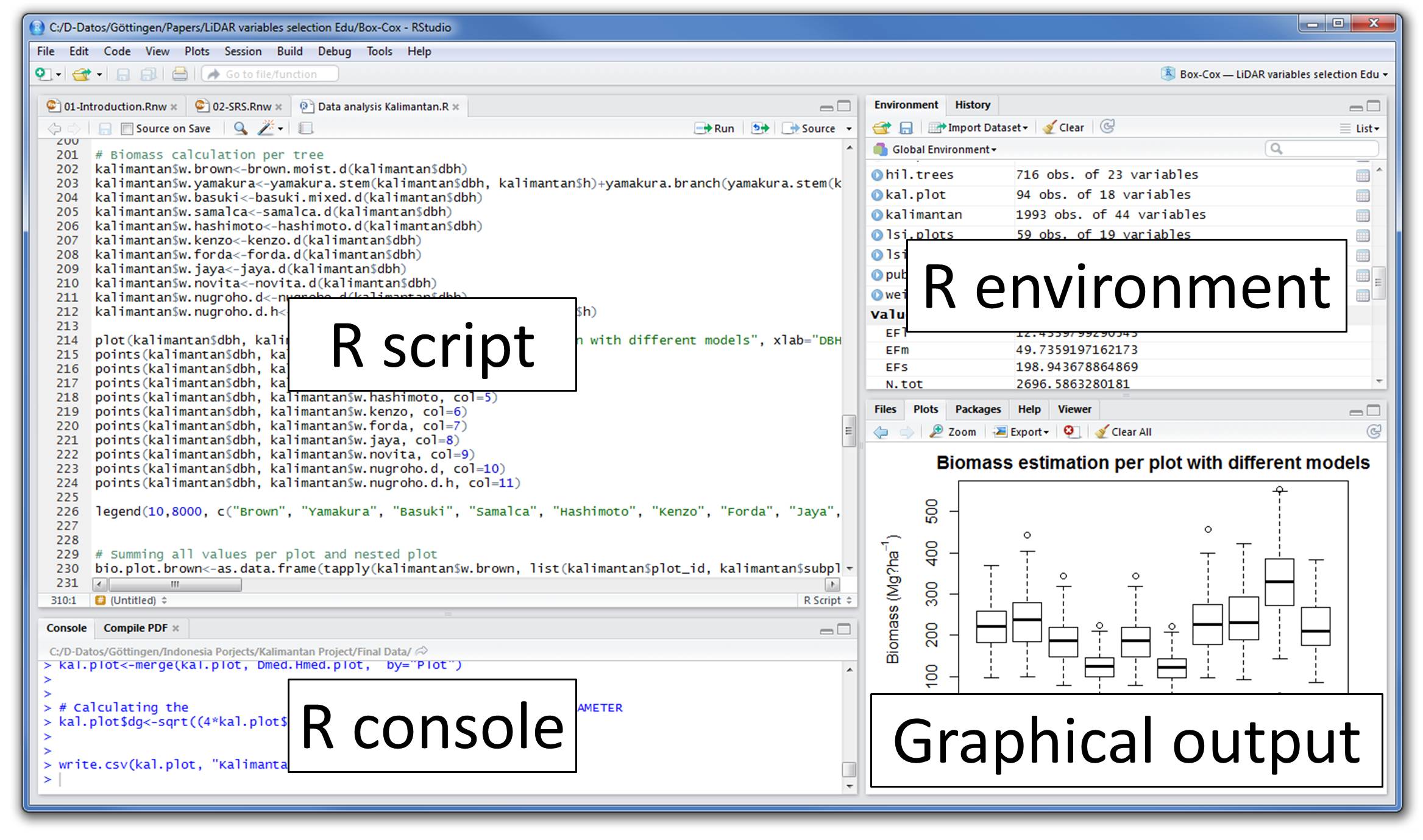
- To Start R Studio, click on its desktop icon or use ‘search windows’ to access the program. It looks like this:
Let’s quickly understand the interface of R Studio:
- R Console: This area shows the output of code you run. Also, you can directly write codes in console. Code entered directly in R console cannot be traced later. This is where R script comes to use.
- R Script: As the name suggest, here you get space to write codes. To run those codes, simply select the line(s) of code and press Ctrl + Enter. Alternatively, you can click on little ‘Run’ button location at top right corner of R Script.
- R environment: This space displays the set of external elements added. This includes data set, variables, vectors, functions etc. To check if data has been loaded properly in R, always look at this area.
- Graphical Output: This space display the graphs created during exploratory data analysis. Not just graphs, you could select packages, seek help with embedded R’s official documentation.
How to install R Packages ?
The sheer power of R lies in its incredible packages. In R, most data handling tasks can be performed in 2 ways: Using R packages and R base functions. In this tutorial, I’ll also introduce you with the most handy and powerful R packages. To install a package, simply type:
install.packages("package name")
As a first time user, a pop might appear to select your CRAN mirror (country server), choose accordingly and press OK.
Note: You can type this either in console directly and press ‘Enter’ or in R script and click ‘Run’.
Basic Computations in R
Let’s begin with basics. To get familiar with R coding environment, start with some basic calculations. R console can be used as an interactive calculator too. Type the following in your console:
> 2 + 3
> 5
> 6 / 3
> 2
> (3*8)/(2*3)
> 4
> log(12)
> 1.07
> sqrt (121)
> 11
Similarly, you can experiment various combinations of calculations and get the results. In case, you want to obtain the previous calculation, this can be done in two ways. First, click in R console, and press ‘Up / Down Arrow’ key on your keyboard. This will activate the previously executed commands. Press Enter.
But, what if you have done too many calculations ? It would be too painful to scroll through every command and find it out. In such situations, creating variable is a helpful way.
In R, you can create a variable using <- or = sign. Let’s say I want to create a variable x to compute the sum of 7 and 8. I’ll write it as:
> x <- 8 + 7
> x

> 15
Once we create a variable, you no longer get the output directly (like calculator), unless you call the variable in the next line. Remember, variables can be alphabets, alphanumeric but not numeric. You can’t create numeric variables.
2. Essentials of R Programming
Understand and practice this section thoroughly. This is the building block of your R programming knowledge. If you get this right, you would face less trouble in debugging.
R has five basic or ‘atomic’ classes of objects. Wait, what is an object ?
Everything you see or create in R is an object. A vector, matrix, data frame, even a variable is an object. R treats it that way. So, R has 5 basic classes of objects. This includes:
- Character
- Numeric (Real Numbers)
- Integer (Whole Numbers)
- Complex
- Logical (True / False)
Since these classes are self-explanatory by names, I wouldn’t elaborate on that. These classes have attributes. Think of attributes as their ‘identifier’, a name or number which aptly identifies them. An object can have following attributes:
- names, dimension names
- dimensions
- class
- length
Attributes of an object can be accessed using attributes() function. More on this coming in following section.
Let’s understand the concept of object and attributes practically. The most basic object in R is known as vector. You can create an empty vector using vector(). Remember, a vector contains object of same class.
For example: Let’s create vectors of different classes. We can create vector using c() or concatenate command also.
> a <- c(1.8, 4.5) #numeric
> b <- c(1 + 2i, 3 - 6i) #complex
> d <- c(23, 44)   #integer

> e <- vector("logical", length = 5)
Similarly, you can create vector of various classes.
Data Types in R
R has various type of ‘data types’ which includes vector (numeric, integer etc), matrices, data frames and list. Let’s understand them one by one.
Vector: As mentioned above, a vector contains object of same class. But, you can mix objects of different classes too. When objects of different classes are mixed in a list, coercion occurs. This effect causes the objects of different types to ‘convert’ into one class. For example:
> qt <- c("Time", 24, "October", TRUE, 3.33)  #character

> ab <- c(TRUE, 24) #numeric

> cd <- c(2.5, "May") #character
To check the class of any object, use class(“vector name”) function.
> class(qt)
"character"
To convert the class of a vector, you can use as. command.
> bar <- 0:5
> class(bar)
> "integer"
> as.numeric(bar)
> class(bar)
> "numeric"
> as.character(bar)
> class(bar)
> "character"
Similarly, you can change the class of any vector. But, you should pay attention here. If you try to convert a “character” vector to “numeric” , NAs will be introduced. Hence, you should be careful to use this command.
List: A list is a special type of vector which contain elements of different data types. For example:
> my_list <- list(22, "ab", TRUE, 1 + 2i)
> my_list
[[1]]
[1] 22
[[2]]
[1] "ab"
[[3]]
[1] TRUE
[[4]]
[1] 1+2i
As you can see, the output of a list is different from a vector. This is because, all the objects are of different types. The double bracket [[1]] shows the index of first element and so on. Hence, you can easily extract the element of lists depending on their index. Like this:
> my_list[[3]]
> [1] TRUE
You can use [] single bracket too. But, that would return the list element with its index number, instead of the result above. Like this:
> my_list[3]
> [[1]]
[1] TRUE
Matrices: When a vector is introduced with row and column i.e. a dimension attribute, it becomes a matrix. A matrix is represented by set of rows and columns. It is a 2 dimensional data structure. It consist of elements of same class. Let’s create a matrix of 3 rows and 2 columns:
> my_matrix <- matrix(1:6, nrow=3, ncol=2)
> my_matrix
[,1] [,2]
[1,] 1 4
[2,] 2 5
[3,] 3 6
> dim(my_matrix)
[1] 3 2
> attributes(my_matrix)
$dim
[1] 3 2
As you can see, the dimensions of a matrix can be obtained using either dim() or attributes() command. To extract a particular element from a matrix, simply use the index shown above. For example(try this at your end):
> my_matrix[,2] #extracts second column
> my_matrix[,1] #extracts first column
> my_matrix[2,] #extracts second row
> my_matrix[1,] #extracts first row
As an interesting fact, you can also create a matrix from a vector. All you need to do is, assign dimension dim() later. Like this:
> age <- c(23, 44, 15, 12, 31, 16)
> age
[1] 23 44 15 12 31 16
> dim(age) <- c(2,3)
> age
[,1] [,2] [,3]
[1,] 23 15 31
[2,] 44 12 16
> class(age)
[1] "matrix"
You can also join two vectors using cbind() and rbind() functions. But, make sure that both vectors have same number of elements. If not, it will return NA values.
> x <- c(1, 2, 3, 4, 5, 6)
> y <- c(20, 30, 40, 50, 60)
> cbind(x, y)
> cbind(x, y)

x    y

[1,] 1 20

[2,] 2 30

[3,] 3 40

[4,] 4 50

[5,] 5 60

[6,] 6 70
> class(cbind(x, y))
[1] “matrix”
Data Frame: This is the most commonly used member of data types family. It is used to store tabular data. It is different from matrix. In a matrix, every element must have same class. But, in a data frame, you can put list of vectors containing different classes. This means, every column of a data frame acts like a list. Every time you will read data in R, it will be stored in the form of a data frame. Hence, it is important to understand the majorly used commands on data frame:
> df <- data.frame(name = c("ash","jane","paul","mark"), score = c(67,56,87,91))
> df
name score
1 ash 67
2 jane 56
3 paul 87
4 mark 91
> dim(df)
[1] 4 2
> str(df)
'data.frame': 4 obs. of 2 variables:
$ name : Factor w/ 4 levels "ash","jane","mark",..: 1 2 4 3
$ score: num 67 56 87 91
> nrow(df)
[1] 4
> ncol(df)
[1] 2
Let’s understand the code above. df is the name of data frame. dim() returns the dimension of data frame as 4 rows and 2 columns. str() returns the structure of a data frame i.e. the list of variables stored in the data frame. nrow() and ncol() return the number of rows and number of columns in a data set respectively.
Here you see “name” is a factor variable and “score” is numeric. In data science, a variable can be categorized into two types: Continuous and Categorical.
Continuous variables are those which can take any form such as 1, 2, 3.5, 4.66 etc. Categorical variables are those which takes only discrete values such as 2, 5, 11, 15 etc. In R, categorical values are represented by factors. In df, name is a factor variable having 4 unique levels. Factor or categorical variable are specially treated in a data set. For more explanation, click here. Similarly, you can find techniques to deal with continuous variables here.
Let’s now understand the concept of missing values in R. This is one of the most painful yet crucial part of predictive modeling. You must be aware of all techniques to deal with them. The complete explanation on such techniques is provided here.
Missing values in R are represented by NA and NaN. Now we’ll check if a data set has missing values (using the same data frame df).
> df[1:2,2] <- NA #injecting NA at 1st, 2nd row and 2nd column of df
> df
name score
1 ash NA
2 jane NA
3 paul 87
4 mark 91
> is.na(df) #checks the entire data set for NAs and return logical output
name score
[1,] FALSE TRUE
[2,] FALSE TRUE
[3,] FALSE FALSE
[4,] FALSE FALSE
> table(is.na(df)) #returns a table of logical output
FALSE TRUE
6 2
> df[!complete.cases(df),] #returns the list of rows having missing values
name score
1 ash NA
2 jane NA
Missing values hinder normal calculations in a data set. For example, let’s say, we want to compute the mean of score. Since there are two missing values, it can’t be done directly. Let’s see:
mean(df$score)
[1] NA
> mean(df$score, na.rm = TRUE)
[1] 89
The use of na.rm = TRUE parameter tells R to ignore the NAs and compute the mean of remaining values in the selected column (score). To remove rows with NA values in a data frame, you can use na.omit:
> new_df <- na.omit(df)
> new_df
name score
3 paul 87
4 mark 91
Control Structures in R
As the name suggest, a control structure ‘controls’ the flow of code / commands written inside a function. A function is a set of multiple commands written to automate a repetitive coding task.
For example: You have 10 data sets. You want to find the mean of ‘Age’ column present in every data set. This can be done in 2 ways: either you write the code to compute mean 10 times or you simply create a function and pass the data set to it.
Let’s understand the control structures in R with simple examples:
if, else – This structure is used to test a condition. Below is the syntax:
if (<condition>){
##do something
} else {
##do something
}
Example
#initialize a variable
N <- 10
#check if this variable * 5 is > 40
if (N * 5 > 40){
print("This is easy!")
} else {
print ("It's not easy!")
}
[1] "This is easy!"
for – This structure is used when a loop is to be executed fixed number of times. It is commonly used for iterating over the elements of an object (list, vector). Below is the syntax:
for (<search condition>){
#do something
}
Example
#initialize a vector
y <- c(99,45,34,65,76,23)
#print the first 4 numbers of this vector
for(i in 1:4){
print (y[i])
}

[1] 99

[1] 45

[1] 34

[1] 65
while – It begins by testing a condition, and executes only if the condition is found to be true. Once the loop is executed, the condition is tested again. Hence, it’s necessary to alter the condition such that the loop doesn’t go infinity. Below is the syntax:
#initialize a condition
Age <- 12
#check if age is less than 17
while(Age < 17){
print(Age)
Age <- Age + 1 #Once the loop is executed, this code breaks the loop
}

[1] 12

[1] 13

[1] 14

[1] 15

[1] 16
There are other control structures as well but are less frequently used than explained above. Those structures are:
- repeat – It executes an infinite loop
- break – It breaks the execution of a loop
- next – It allows to skip an iteration in a loop
- return – It help to exit a function
Note: If you find the section ‘control structures’ difficult to understand, not to worry. R is supported by various packages to compliment the work done by control structures.
Useful R Packages
Out of ~7800 packages listed on CRAN, I’ve listed some of the most powerful and commonly used packages in predictive modeling in this article. Since, I’ve already explained the method of installing packages, you can go ahead and install them now. Sooner or later you’ll need them.
Importing Data: R offers wide range of packages for importing data available in any format such as .txt, .csv, .json, .sql etc. To import large files of data quickly, it is advisable to install and use data.table, readr, RMySQL, sqldf, jsonlite.
Data Visualization: R has in built plotting commands as well. They are good to create simple graphs. But, becomes complex when it comes to creating advanced graphics. Hence, you should install ggplot2.
Data Manipulation: R has a fantastic collection of packages for data manipulation. These packages allows you to do basic & advanced computations quickly. These packages are dplyr, plyr, tidyr, lubridate, stringr. Check out this complete tutorial on data manipulation packages in R.
Modeling / Machine Learning: For modeling, caret package in R is powerful enough to cater to every need for creating machine learning model. However, you can install packages algorithms wise such as randomForest, rpart, gbm etc
Note: I’ve only mentioned the commonly used packages. You might like to check this interesting infographic on complete list of useful R packages.
Till here, you became familiar with the basic work style in R and its associated components. From next section, we’ll begin with predictive modeling. But before you proceed. I want you to practice, what you’ve learnt till here.
Practice Assignment: As a part of this assignment, install ‘swirl’ package in package. Then type, library(swirl) to initiate the package. And, complete this interactive R tutorial. If you have followed this article thoroughly, this assignment should be an easy task for you!
3. Exploratory Data Analysis in R
From this section onwards, we’ll dive deep into various stages of predictive modeling. Hence, make sure you understand every aspect of this section. In case you find anything difficult to understand, ask me in the comments section below.
Data Exploration is a crucial stage of predictive model. You can’t build great and practical models unless you learn to explore the data from begin to end. This stage forms a concrete foundation for data manipulation (the very next stage). Let’s understand it in R.
In this tutorial, I’ve taken the data set from Big Mart Sales Prediction. Before we start, you must get familiar with these terms:
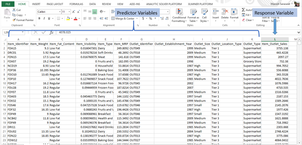
Response Variable (a.k.a Dependent Variable): In a data set, the response variable (y) is one on which we make predictions. In this case, we’ll predict ‘Item_Outlet_Sales’. (Refer to image shown below)
Predictor Variable (a.k.a Independent Variable): In a data set, predictor variables (Xi) are those using which the prediction is made on response variable. (Image below).
Train Data: The predictive model is always built on train data set. An intuitive way to identify the train data is, that it always has the ‘response variable’ included.
Test Data: Once the model is built, it’s accuracy is ‘tested’ on test data. This data always contains less number of observations than train data set. Also, it does not include ‘response variable’.
Right now, you should download the data set. Take a good look at train and test data. Cross check the information shared above and then proceed.
Let’s now begin with importing and exploring data.
#working directory
path <- ".../Data/BigMartSales"
#set working directory
setwd(path)
As a beginner, I’ll advise you to keep the train and test files in your working directly to avoid unnecessary directory troubles. Once the directory is set, we can easily import the .csv files using commands below.
#Load Datasets
train <- read.csv("Train_UWu5bXk.csv")
test <- read.csv("Test_u94Q5KV.csv")
In fact, even prior to loading data in R, it’s a good practice to look at the data in Excel. This helps in strategizing the complete prediction modeling process. To check if the data set has been loaded successfully, look at R environment. The data can be seen there. Let’s explore the data quickly.
#check dimesions ( number of row & columns) in data set
> dim(train)
[1] 8523 12
> dim(test)
[1] 5681 11
We have 8523 rows and 12 columns in train data set and 5681 rows and 11 columns in data set. This makes sense. Test data should always have one column less (mentioned above right?). Let’s get deeper in train data set now.
#check the variables and their types in train
> str(train)
'data.frame': 8523 obs. of 12 variables:
$ Item_Identifier : Factor w/ 1559 levels "DRA12","DRA24",..: 157 9 663 1122 1298 759 697 739 441 991 ...
$ Item_Weight : num 9.3 5.92 17.5 19.2 8.93 ...
$ Item_Fat_Content : Factor w/ 5 levels "LF","low fat",..: 3 5 3 5 3 5 5 3 5 5 ...
$ Item_Visibility : num 0.016 0.0193 0.0168 0 0 ...
$ Item_Type : Factor w/ 16 levels "Baking Goods",..: 5 15 11 7 10 1 14 14 6 6 ...
$ Item_MRP : num 249.8 48.3 141.6 182.1 53.9 ...
$ Outlet_Identifier : Factor w/ 10 levels "OUT010","OUT013",..: 10 4 10 1 2 4 2 6 8 3 ...
$ Outlet_Establishment_Year: int 1999 2009 1999 1998 1987 2009 1987 1985 2002 2007 ...
$ Outlet_Size : Factor w/ 4 levels "","High","Medium",..: 3 3 3 1 2 3 2 3 1 1 ...
$ Outlet_Location_Type : Factor w/ 3 levels "Tier 1","Tier 2",..: 1 3 1 3 3 3 3 3 2 2 ...
$ Outlet_Type : Factor w/ 4 levels "Grocery Store",..: 2 3 2 1 2 3 2 4 2 2 ...
$ Item_Outlet_Sales : num 3735 443 2097 732 995 ...
Let’s do some quick data exploration.
To begin with, I’ll first check if this data has missing values. This can be done by using:
> table(is.na(train))
FALSE TRUE
100813 1463
In train data set, we have 1463 missing values. Let’s check the variables in which these values are missing. It’s important to find and locate these missing values. Many data scientists have repeatedly advised beginners to pay close attention to missing value in data exploration stages.
> colSums(is.na(train))
Item_Identifier Item_Weight
0 1463
Item_Fat_Content Item_Visibility
0 0
Item_Type Item_MRP
0 0
Outlet_Identifier Outlet_Establishment_Year
0 0
Outlet_Size Outlet_Location_Type
0 0
Outlet_Type Item_Outlet_Sales
0 0
Hence, we see that column Item_Weight has 1463 missing values. Let’s get more inferences from this data.
> summary(train)
Here are some quick inferences drawn from variables in train data set:
- Item_Fat_Content has mis-matched factor levels.
- Minimum value of item_visibility is 0. Practically, this is not possible. If an item occupies shelf space in a grocery store, it ought to have some visibility. We’ll treat all 0’s as missing values.
- Item_Weight has 1463 missing values (already explained above).
- Outlet_Size has a unmatched factor levels.
These inference will help us in treating these variable more accurately.
Graphical Representation of Variables
I’m sure you would understand these variables better when explained visually. Using graphs, we can analyze the data in 2 ways: Univariate Analysis and Bivariate Analysis.
Univariate analysis is done with one variable. Bivariate analysis is done with two variables. Univariate analysis is a lot easy to do. Hence, I’ll skip that part here. I’d recommend you to try it at your end. Let’s now experiment doing bivariate analysis and carve out hidden insights.
For visualization, I’ll use ggplot2 package. These graphs would help us understand the distribution and frequency of variables in the data set.
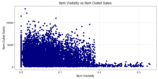
> ggplot(train, aes(x= Item_Visibility, y = Item_Outlet_Sales)) + geom_point(size = 2.5, color="navy") + xlab("Item Visibility") + ylab("Item Outlet Sales") + ggtitle("Item Visibility vs Item Outlet Sales")
We can see that majority of sales has been obtained from products having visibility less than 0.2. This suggests that item_visibility < 2 must be an important factor in determining sales. Let’s plot few more interesting graphs and explore such hidden stories.
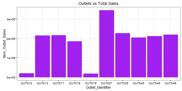
> ggplot(train, aes(Outlet_Identifier, Item_Outlet_Sales)) + geom_bar(stat = "identity", color = "purple") +theme(axis.text.x = element_text(angle = 70, vjust = 0.5, color = "black")) + ggtitle("Outlets vs Total Sales") + theme_bw()
Here, we infer that OUT027 has contributed to majority of sales followed by OUT35. OUT10 and OUT19 have probably the least footfall, thereby contributing to the least outlet sales.
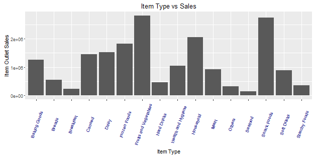
> ggplot(train, aes(Item_Type, Item_Outlet_Sales)) + geom_bar( stat = "identity") +theme(axis.text.x = element_text(angle = 70, vjust = 0.5, color = "navy")) + xlab("Item Type") + ylab("Item Outlet Sales")+ggtitle("Item Type vs Sales")
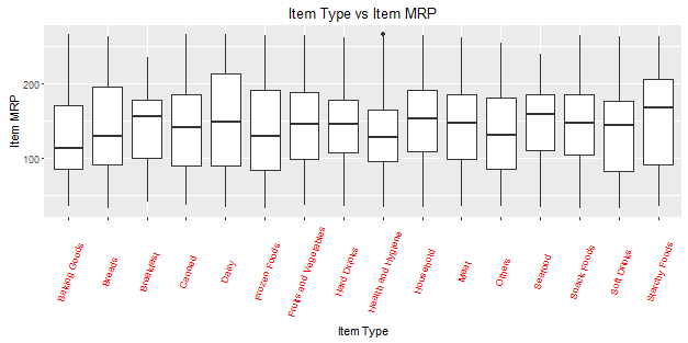
From this graph, we can infer that Fruits and Vegetables contribute to the highest amount of outlet sales followed by snack foods and household products. This information can also be represented using a box plot chart. The benefit of using a box plot is, you get to see the outlier and mean deviation of corresponding levels of a variable (shown below).
> ggplot(train, aes(Item_Type, Item_MRP)) +geom_boxplot() +ggtitle("Box Plot") + theme(axis.text.x = element_text(angle = 70, vjust = 0.5, color = "red")) + xlab("Item Type") + ylab("Item MRP") + ggtitle("Item Type vs Item MRP")
The black point you see, is an outlier. The mid line you see in the box, is the mean value of each item type. To know more about boxplots, check this tutorial.
Now, we have an idea of the variables and their importance on response variable. Let’s now move back to where we started. Missing values. Now we’ll impute the missing values.
We saw variable Item_Weight has missing values. Item_Weight is an continuous variable. Hence, in this case we can impute missing values with mean / median of item_weight. These are the most commonly used methods of imputing missing value. To explore other methods of this techniques, check out this tutorial.
Let’s first combine the data sets. This will save our time as we don’t need to write separate codes for train and test data sets. To combine the two data frames, we must make sure that they have equal columns, which is not the case.
> dim(train)
[1] 8523 12
> dim(test)
[1] 5681 11
Test data set has one less column (response variable). Let’s first add the column. We can give this column any value. An intuitive approach would be to extract the mean value of sales from train data set and use it as placeholder for test variable Item _Outlet_ Sales. Anyways, let’s make it simple for now. I’ve taken a value 1. Now, we’ll combine the data sets.
> test$Item_Outlet_Sales <- 1
> combi <- rbind(train, test)
Impute missing value by median. I’m using median because it is known to be highly robust to outliers. Moreover, for this problem, our evaluation metric is RMSE which is also highly affected by outliers. Hence, median is better in this case.
> combi$Item_Weight[is.na(combi$Item_Weight)] <- median(combi$Item_Weight, na.rm = TRUE)
> table(is.na(combi$Item_Weight))
FALSE
14204
Trouble with Continuous Variables & Categorical Variables
It’s important to learn to deal with continuous and categorical variables separately in a data set. In other words, they need special attention. In this data set, we have only 3 continuous variables and rest are categorical in nature. If you are still confused, I’ll suggest you to once again look at the data set using str() and proceed.
Let’s take up Item_Visibility. In the graph above, we saw item visibility has zero value also, which is practically not feasible. Hence, we’ll consider it as a missing value and once again make the imputation using median.
> combi$Item_Visibility <- ifelse(combi$Item_Visibility == 0,
median(combi$Item_Visibility), combi$Item_Visibility)
Let’s proceed to categorical variables now. During exploration, we saw there are mis-matched levels in variables which needs to be corrected.
> levels(combi$Outlet_Size)[1] <- "Other"
> library(plyr)
> combi$Item_Fat_Content <- revalue(combi$Item_Fat_Content,

c("LF" = "Low Fat", "reg" = "Regular"))

> combi$Item_Fat_Content <- revalue(combi$Item_Fat_Content, c("low fat" = "Low Fat"))
> table(combi$Item_Fat_Content)
Low Fat Regular
9185 5019
Using the commands above, I’ve assigned the name ‘Other’ to unnamed level in Outlet_Size variable. Rest, I’ve simply renamed the various levels of Item_Fat_Content.
4. Data Manipulation in R
Let’s call it as, the advanced level of data exploration. In this section we’ll practically learn about feature engineering and other useful aspects.
Feature Engineering: This component separates an intelligent data scientist from a technically enabled data scientist. You might have access to large machines to run heavy computations and algorithms, but the power delivered by new features, just can’t be matched. We create new variables to extract and provide as much ‘new’ information to the model, to help it make accurate predictions.
If you have been thinking all this time, great. But now is the time to think deeper. Look at the data set and ask yourself, what else (factor) could influence Item_Outlet_Sales ? Anyhow, the answer is below. But, I want you to try it out first, before scrolling down.
1. Count of Outlet Identifiers – There are 10 unique outlets in this data. This variable will give us information on count of outlets in the data set. More the number of counts of an outlet, chances are more will be the sales contributed by it.
> library(dplyr)
> a <- combi%>%
group_by(Outlet_Identifier)%>%
tally()
> head(a)
Source: local data frame [6 x 2]
Outlet_Identifier n
(fctr) (int)
1 OUT010 925
2 OUT013 1553
3 OUT017 1543
4 OUT018 1546
5 OUT019 880
6 OUT027 1559
> names(a)[2] <- "Outlet_Count"
> combi <- full_join(a, combi, by = "Outlet_Identifier")
As you can see, dplyr package makes data manipulation quite effortless. You no longer need to write long function. In the code above, I’ve simply stored the new data frame in a variable a. Later, the new column Outlet_Count is added in our original ‘combi’ data set. To know more about dplyr, follow this tutorial.
2. Count of Item Identifiers – Similarly, we can compute count of item identifiers too. It’s a good practice to fetch more information from unique ID variables using their count. This will help us to understand, which outlet has maximum frequency.
> b <- combi%>%
group_by(Item_Identifier)%>%
tally()
> names(b)[2] <- "Item_Count"

> head (b)

Item_Identifier   Item_Count

(fctr)            (int)

1 DRA12             9

2 DRA24             10

3 DRA59             10

4 DRB01             8

5 DRB13             9

6 DRB24             8
> combi <- merge(b, combi, by = “Item_Identifier”)
3. Outlet Years – This variable represent the information of existence of a particular outlet since year 2013. Why just 2013? You’ll find the answer in problem statement here. My hypothesis is, older the outlet, more footfall, large base of loyal customers and larger the outlet sales.
> c <- combi%>%
select(Outlet_Establishment_Year)%>%
mutate(Outlet_Year = 2013 - combi$Outlet_Establishment_Year)
> head(c)
Outlet_Establishment_Year Outlet_Year
1 1999 14
2 2009 4
3 1999 14
4 1998 15
5 1987 26
6 2009 4
> combi <- full_join(c, combi)
This suggests that outlets established in 1999 were 14 years old in 2013 and so on.
4. Item Type New – Now, pay attention to Item_Identifiers. We are about to discover a new trend. Look carefully, there is a pattern in the identifiers starting with “FD”,”DR”,”NC”. Now, check the corresponding Item_Types to these identifiers in the data set. You’ll discover, items corresponding to “DR”, are mostly eatables. Items corresponding to “FD”, are drinks. And, item corresponding to “NC”, are products which can’t be consumed, let’s call them non-consumable. Let’s extract these variables into a new variable representing their counts.
Here I’ll use substr(), gsub() function to extract and rename the variables respectively.
> q <- substr(combi$Item_Identifier,1,2)
> q <- gsub("FD","Food",q)
> q <- gsub("DR","Drinks",q)
> q <- gsub("NC","Non-Consumable",q)
> table(q)
Drinks Food Non-Consumable
1317 10201 2686
Let’s now add this information in our data set with a variable name ‘Item_Type_New.
> combi$Item_Type_New <- q
I’ll leave the rest of feature engineering intuition to you. You can think of more variables which could add more information to the model. But make sure, the variable aren’t correlated. Since, they are emanating from a same set of variable, there is a high chance for them to be correlated. You can check the same in R using cor() function.
Label Encoding and One Hot Encoding
Just, one last aspect of feature engineering left. Label Encoding and One Hot Encoding.
Label Encoding, in simple words, is the practice of numerically encoding (replacing) different levels of a categorical variables. For example: In our data set, the variable Item_Fat_Content has 2 levels: Low Fat and Regular. So, we’ll encode Low Fat as 0 and Regular as 1. This will help us convert a factor variable in numeric variable. This can be simply done using if else statement in R.
> combi$Item_Fat_Content <- ifelse(combi$Item_Fat_Content == "Regular",1,0)
One Hot Encoding, in simple words, is the splitting a categorical variable into its unique levels, and eventually removing the original variable from data set. Confused ? Here’s an example: Let’s take any categorical variable, say, Outlet_ Location_Type. It has 3 levels. One hot encoding of this variable, will create 3 different variables consisting of 1s and 0s. 1s will represent the existence of variable and 0s will represent non-existence of variable. Let look at a sample:
> sample <- select(combi, Outlet_Location_Type)
> demo_sample <- data.frame(model.matrix(~.-1,sample))

> head(demo_sample)

Outlet_Location_TypeTier.1 Outlet_Location_TypeTier.2 Outlet_Location_TypeTier.3

1             1                         0                        0

2             0                         0                        1

3             1                         0                        0

4             0                         0                        1

5             0                         0                        1

6             0                         0                        1
model.matrix creates a matrix of encoded variables. ~. -1 tells R, to encode all variables in the data frame, but suppress the intercept. So, what will happen if you don’t write -1 ? model.matrix will skip the first level of the factor, thereby resulting in just 2 out of 3 factor levels (loss of information).
This was the demonstration of one hot encoding. Hope you have understood the concept now. Let’s now apply this technique to all categorical variables in our data set (excluding ID variable).
>library(dummies)

>combi <- dummy.data.frame(combi, names = c('Outlet_Size','Outlet_Location_Type','Outlet_Type', 'Item_Type_New'),  sep='_')
With this, I have shared 2 different methods of performing one hot encoding in R. Let’s check if encoding has been done.
> str (combi)
$ Outlet_Size_Other : int 0 1 1 0 1 0 0 0 0 0 ...
$ Outlet_Size_High : int 0 0 0 1 0 0 0 0 0 0 ...
$ Outlet_Size_Medium : int 1 0 0 0 0 0 1 1 0 1 ...
$ Outlet_Size_Small : int 0 0 0 0 0 1 0 0 1 0 ...
$ Outlet_Location_Type_Tier 1 : int 1 0 0 0 0 0 0 0 1 0 ...
$ Outlet_Location_Type_Tier 2 : int 0 1 0 0 1 1 0 0 0 0 ...
$ Outlet_Location_Type_Tier 3 : int 0 0 1 1 0 0 1 1 0 1 ...
$ Outlet_Type_Grocery Store : int 0 0 1 0 0 0 0 0 0 0 ...
$ Outlet_Type_Supermarket Type1: int 1 1 0 1 1 1 0 0 1 0 ...
$ Outlet_Type_Supermarket Type2: int 0 0 0 0 0 0 0 1 0 0 ...
$ Outlet_Type_Supermarket Type3: int 0 0 0 0 0 0 1 0 0 1 ...
$ Item_Outlet_Sales : num 1 3829 284 2553 2553 ...
$ Year : num 14 11 15 26 6 9 28 4 16 28 ...
$ Item_Type_New_Drinks : int 1 1 1 1 1 1 1 1 1 1 ...
$ Item_Type_New_Food : int 0 0 0 0 0 0 0 0 0 0 ...
$ Item_Type_New_Non-Consumable : int 0 0 0 0 0 0 0 0 0 0 ...
As you can see, after one hot encoding, the original variables are removed automatically from the data set.
5. Predictive Modeling using Machine Learning
Finally, we’ll drop the columns which have either been converted using other variables or are identifier variables. This can be accomplished using select from dplyr package.
> combi <- select(combi, -c(Item_Identifier, Outlet_Identifier, Item_Fat_Content, Outlet_Establishment_Year,Item_Type))
> str(combi)
In this section, I’ll cover Regression, Decision Trees and Random Forest. A detailed explanation of these algorithms is outside the scope of this article. These algorithms have been satisfactorily explained in our previous articles. I’ve provided the links for useful resources.
As you can see, we have encoded all our categorical variables. Now, this data set is good to take forward to modeling. Since, we started from Train and Test, let’s now divide the data sets.
> new_train <- combi[1:nrow(train),]
> new_test <- combi[-(1:nrow(train)),]
Linear (Multiple) Regression
Multiple Regression is used when response variable is continuous in nature and predictors are many. Had it been categorical, we would have used Logistic Regression. Before you proceed, sharpen your basics of Regression here.
Linear Regression takes following assumptions:
- There exists a linear relationship between response and predictor variables
- The predictor (independent) variables are not correlated with each other. Presence of collinearity leads to a phenomenon known as multicollinearity.
- The error terms are uncorrelated. Otherwise, it will lead to autocorrelation.
- Error terms must have constant variance. Non-constant variance leads to heteroskedasticity.
Let’s now build out first regression model on this data set. R uses lm() function for regression.
> linear_model <- lm(Item_Outlet_Sales ~ ., data = new_train)
> summary(linear_model)
Adjusted R² measures the goodness of fit of a regression model. Higher the R², better is the model. Our R² = 0.2085. It means we really did something drastically wrong. Let’s figure it out.
In our case, I could find our new variables aren’t helping much i.e. Item count, Outlet Count and Item_Type_New. Neither of these variables are significant. Significant variables are denoted by ‘*’ sign.
As we know, correlated predictor variables brings down the model accuracy. Let’s find out the amount of correlation present in our predictor variables. This can be simply calculated using:
> cor(new_train)
Alternatively, you can also use corrplot package for some fancy correlation plots. Scrolling through the long list of correlation coefficients, I could find a deadly correlation coefficient:
cor(new_train$Outlet_Count, new_train$`Outlet_Type_Grocery Store`)
[1] -0.9991203
Outlet_Count is highly correlated (negatively) with Outlet Type Grocery Store. Here are some problems I could find in this model:
- We have correlated predictor variables.
- We did one hot encoding and label encoding. That’s not necessary since linear regression handle categorical variables by creating dummy variables intrinsically.
- The new variables (item count, outlet count, item type new) created in feature engineering are not significant.
Let’s try to create a more robust regression model. This time, I’ll be using a building a simple model without encoding and new features. Below is the entire code:
#load directory
> path <- "C:/Users/manish/desktop/Data/February 2016"
> setwd(path)
#load data
> train <- read.csv("train_Big.csv")
> test <- read.csv("test_Big.csv")
#create a new variable in test file
> test$Item_Outlet_Sales <- 1
#combine train and test data
> combi <- rbind(train, test)
#impute missing value in Item_Weight
> combi$Item_Weight[is.na(combi$Item_Weight)] <- median(combi$Item_Weight, na.rm = TRUE)
#impute 0 in item_visibility
> combi$Item_Visibility <- ifelse(combi$Item_Visibility == 0, median(combi$Item_Visibility), combi$Item_Visibility)
#rename level in Outlet_Size
> levels(combi$Outlet_Size)[1] <- "Other"
#rename levels of Item_Fat_Content
> library(plyr)
> combi$Item_Fat_Content <- revalue(combi$Item_Fat_Content,c("LF" = "Low Fat", "reg" = "Regular"))
> combi$Item_Fat_Content <- revalue(combi$Item_Fat_Content, c("low fat" = "Low Fat"))
#create a new column 2013 - Year
> combi$Year <- 2013 - combi$Outlet_Establishment_Year
#drop variables not required in modeling
> library(dplyr)
> combi <- select(combi, -c(Item_Identifier, Outlet_Identifier, Outlet_Establishment_Year))
#divide data set
> new_train <- combi[1:nrow(train),]
> new_test <- combi[-(1:nrow(train)),]
#linear regression
> linear_model <- lm(Item_Outlet_Sales ~ ., data = new_train)
> summary(linear_model)
Now we have got R² = 0.5623. This teaches us that, sometimes all you need is simple thought process to get high accuracy. Quite a good improvement from previous model. Next, time when you work on any model, always remember to start with a simple model.
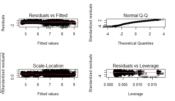
Let’s check out regression plot to find out more ways to improve this model.
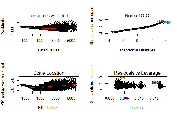
> par(mfrow=c(2,2))
> plot(linear_model)
You can zoom these graphs in R Studio at your end. All these plots have a different story to tell. But the most important story is being portrayed by Residuals vs Fitted graph.
Residual values are the difference between actual and predicted outcome values. Fitted values are the predicted values. If you see carefully, you’ll discover it as a funnel shape graph (from right to left ). The shape of this graph suggests that our model is suffering from heteroskedasticity (unequal variance in error terms). Had there been constant variance, there would be no pattern visible in this graph.
A common practice to tackle heteroskedasticity is by taking the log of response variable. Let’s do it and check if we can get further improvement.
> linear_model <- lm(log(Item_Outlet_Sales) ~ ., data = new_train)
> summary(linear_model)
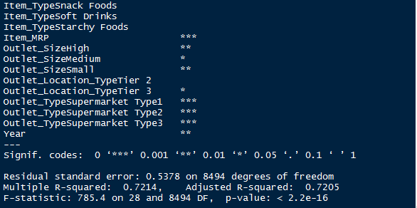
And, here’s a snapshot of my model output. Congrats! We have got an improved model with R² = 0.72. Now, we are on the right path. Once again you can check the residual plots (you might zoom it). You’ll find there is no longer a trend in residual vs fitted value plot.
This model can be further improved by detecting outliers and high leverage points. For now, I leave that part to you! I shall write a separate post on mysteries of regression soon. For now, let’s check our RMSE so that we can compare it with other algorithms demonstrated below.
To calculate RMSE, we can load a package named Metrics.
> install.packages("Metrics")
> library(Metrics)
> rmse(new_train$Item_Outlet_Sales, exp(linear_model$fitted.values))
[1] 1140.004
Let’s proceed to decision tree algorithm and try to improve our RMSE score.
Decision Trees
Before you start, I’d recommend you to glance through the basics of decision tree algorithms. To understand what makes it superior than linear regression, check this tutorial Part 1 and Part 2.
In R, decision tree algorithm can be implemented using rpart package. In addition, we’ll use caret package for doing cross validation. Cross validation is a technique to build robust models which are not prone to overfitting. Read more about Cross Validation.
In R, decision tree uses a complexity parameter (cp). It measures the tradeoff between model complexity and accuracy on training set. A smaller cp will lead to a bigger tree, which might overfit the model. Conversely, a large cp value might underfit the model. Underfitting occurs when the model does not capture underlying trends properly. Let’s find out the optimum cp value for our model with 5 fold cross validation.
#loading required libraries
> library(rpart)
> library(e1071)
> library(rpart.plot)
> library(caret)
#setting the tree control parameters
> fitControl <- trainControl(method = "cv", number = 5)
> cartGrid <- expand.grid(.cp=(1:50)*0.01)
#decision tree
> tree_model <- train(Item_Outlet_Sales ~ ., data = new_train, method = "rpart", trControl = fitControl, tuneGrid = cartGrid)
> print(tree_model)
The final value for cp = 0.01. You can also check the table populated in console for more information. The model with cp = 0.01 has the least RMSE. Let’s now build a decision tree with 0.01 as complexity parameter.
> main_tree <- rpart(Item_Outlet_Sales ~ ., data = new_train, control = rpart.control(cp=0.01))
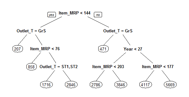
> prp(main_tree)
Here is the tree structure of our model. If you have gone through the basics, you would now understand that this algorithm has marked Item_MRP as the most important variable (being the root node). Let’s check the RMSE of this model and see if this is any better than regression.
> pre_score <- predict(main_tree, type = "vector")
> rmse(new_train$Item_Outlet_Sales, pre_score)
[1] 1102.774
As you can see, our RMSE has further improved from 1140 to 1102.77 with decision tree. To improve this score further, you can further tune the parameters for greater accuracy.
Random Forest
Random Forest is a powerful algorithm which holistically takes care of missing values, outliers and other non-linearities in the data set. It’s simply a collection of classification trees, hence the name ‘forest’. I’d suggest you to quickly refresh your basics of random forest with this tutorial.
In R, random forest algorithm can be implement using randomForest package. Again, we’ll use train package for cross validation and finding optimum value of model parameters.
For this problem, I’ll focus on two parameters of random forest. mtry and ntree. ntree is the number of trees to be grown in the forest. mtry is the number of variables taken at each node to build a tree. And, we’ll do a 5 fold cross validation.
Let’s do it!
#load randomForest library
> library(randomForest)
#set tuning parameters
> control <- trainControl(method = "cv", number = 5)
#random forest model
> rf_model <- train(Item_Outlet_Sales ~ ., data = new_train, method = "parRF", trControl = control, prox = TRUE, allowParallel = TRUE)
#check optimal parameters
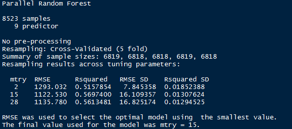
> print(rf_model)
If you notice, you’ll see I’ve used method = “parRF”. This is parallel random forest. This is parallel implementation of random forest. This package causes your local machine to take less time in random forest computation. Alternatively, you can also use method = “rf” as a standard random forest function.
Now we’ve got the optimal value of mtry = 15. Let’s use 1000 trees for computation.
#random forest model
> forest_model <- randomForest(Item_Outlet_Sales ~ ., data = new_train, mtry = 15, ntree = 1000)
> print(forest_model)
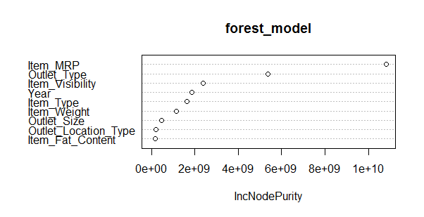
> varImpPlot(forest_model)
This model throws RMSE = 1132.04 which is not an improvement over decision tree model. Random forest has a feature of presenting the important variables. We see that the most important variable is Item_MRP (also shown by decision tree algorithm).
This model can be further improved by tuning parameters. Also, Let’s make out first submission with our best RMSE score by decision tree.
> main_predict <- predict(main_tree, newdata = new_test, type = "vector")
> sub_file <- data.frame(Item_Identifier = test$Item_Identifier, Outlet_Identifier = test$Outlet_Identifier, Item_Outlet_Sales = main_predict)
> write.csv(sub_file, 'Decision_tree_sales.csv')
When predicted on out of sample data, our RMSE has come out to be 1174.33. Here are some things you can do to improve this model further:
- Since we did not use encoding, I encourage you to use one hot encoding and label encoding for random forest model.
- Parameters Tuning will help.
- Use Gradient Boosting.
- Build an ensemble of these models. Read more about Ensemble Modeling.
Do implement the ideas suggested above and share your improvement in the comments section below. Currently, Rank 1 on Leaderboard has obtained RMSE score of 1137.71. Beat it!
End Notes
This brings us to the end of this tutorial. Regret for not so happy ending. But, I’ve given you enough hints to work on. The decision to not use encoded variables in the model, turned out to be beneficial until decision trees.
The motive of this tutorial was to get your started with predictive modeling in R. We learnt few uncanny things such as ‘build simple models’. Don’t jump towards building a complex model. Simple models give you benchmark score and a threshold to work with.
In this tutorial, I have demonstrated the steps used in predictive modeling in R. I’ve covered data exploration, data visualization, data manipulation and building models using Regression, Decision Trees and Random Forest algorithms.
Did you find this tutorial useful ? Are you facing any trouble at any stage of this tutorial ? Feel free to mention your doubts in the comments section below. Do share if you get a better score.
Edit: On visitor’s request, the PDF version of the tutorial is available for download. You need to create a log in account to download the PDF. Also, you can bookmark this page for future reference. Download Here.


