Simple Guide to Logistic Regression in R and Python

Overview

• Get an introduction to logistic regression using R and Python
• Logistic Regression is a popular classification algorithm used to predict a binary outcome
• There are various metrics to evaluate a logistic regression model such as confusion matrix, AUC-ROC curve, etc

Introduction

Every machine learning algorithm works best under a given set of conditions. Making sure your algorithm fits the assumptions/requirements ensures superior performance. You can’t use any algorithm in any condition. For example: Have you ever tried using linear regression on a categorical dependent variable? Don’t even try! Because you won’t be appreciated for getting extremely low values of adjusted R² and F statistic.

Instead, in such situations, you should try using algorithms such as Logistic Regression, Decision Trees, SVM, Random Forest etc. To get a quick overview of these algorithms, I’ll recommend reading – Essentials of Machine Learning Algorithms.

With this post, I give you useful knowledge on Logistic Regression in R. After you’ve mastered linear regression, this comes as the natural following step in your journey. It’s also easy to learn and implement, but you must know the science behind this algorithm.

I’ve tried to explain these concepts in the simplest possible manner. Let’s get started.

What is Logistic Regression?

Logistic Regression is a classification algorithm. It is used to predict a binary outcome (1 / 0, Yes / No, True / False) given a set of independent variables. To represent binary/categorical outcome, we use dummy variables. You can also think of logistic regression as a special case of linear regression when the outcome variable is categorical, where we are using log of odds as dependent variable. In simple words, it predicts the probability of occurrence of an event by fitting data to a logit function.

Derivation of Logistic Regression Equation

Logistic Regression is part of a larger class of algorithms known as Generalized Linear Model (glm). In 1972, Nelder and Wedderburn proposed this model with an effort to provide a means of using linear regression to the problems which were not directly suited for application of linear regression. Infact, they proposed a class of different models (linear regression, ANOVA, Poisson Regression etc) which included logistic regression as a special case.

The fundamental equation of generalized linear model is:

g(E(y)) = α + βx1 + γx2

Here, g() is the link function, E(y) is the expectation of target variable and α + βx1 + γx2 is the linear predictor ( α,β,γ to be predicted). The role of link function is to ‘link’ the expectation of y to linear predictor.

Important Points

1. GLM does not assume a linear relationship between dependent and independent variables. However, it assumes a linear relationship between link function and independent variables in logit model.
2.  The dependent variable need not to be normally distributed.
3. It does not uses OLS (Ordinary Least Square) for parameter estimation. Instead, it uses maximum likelihood estimation (MLE).
4. Errors need to be independent but not normally distributed.

Let’s understand it further using an example:

We are provided a sample of 1000 customers. We need to predict the probability whether a customer will buy (y) a particular magazine or not. As you can see, we’ve a categorical outcome variable, we’ll use logistic regression. Vidalista 20 https://tyackdentalgroup.com/vidalista

To start with logistic regression, I’ll first write the simple linear regression equation with dependent variable enclosed in a link function:

                           g(y) = βo + β(Age)         ---- (a)

Note: For ease of understanding, I’ve considered ‘Age’ as independent variable.

In logistic regression, we are only concerned about the probability of outcome dependent variable ( success or failure). As described above, g() is the link function. This function is established using two things: Probability of Success(p) and Probability of Failure(1-p). p should meet following criteria:

1. It must always be positive (since p >= 0)
2. It must always be less than equals to 1 (since p <= 1)

Now, we’ll simply satisfy these 2 conditions and get to the core of logistic regression. To establish link function, we’ll denote g() with ‘p’ initially and eventually end up deriving this function.

Since probability must always be positive, we’ll put the linear equation in exponential form. For any value of slope and dependent variable, exponent of this equation will never be negative.

p = exp(βo + β(Age)) = e^(βo + β(Age))    ------- (b)

To make the probability less than 1, we must divide p by a number greater than p. This can simply be done by:

p  =  exp(βo + β(Age)) / exp(βo + β(Age)) + 1   =   e^(βo + β(Age)) / e^(βo + β(Age)) + 1    ----- (c)

Using (a), (b) and (c), we can redefine the probability as:

              p = e^y/ 1 + e^y           --- (d)

where p is the probability of success. This (d) is the Logit Function

If p is the probability of success, 1-p will be the probability of failure which can be written as:

q = 1 - p = 1 - (e^y/ 1 + e^y)    --- (e)

where q is the probability of failure

On dividing, (d) / (e), we get,

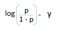
After taking log on both side, we get,

log(p/1-p) is the link function. Logarithmic transformation on the outcome variable allows us to model a non-linear association in a linear way.

After substituting value of y, we’ll get:

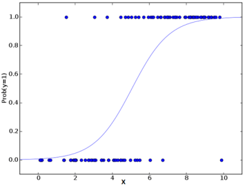
This is the equation used in Logistic Regression. Here (p/1-p) is the odd ratio. Whenever the log of odd ratio is found to be positive, the probability of success is always more than 50%. A typical logistic model plot is shown below. You can see probability never goes below 0 and above 1.

Performance of Logistic Regression Model

To evaluate the performance of a logistic regression model, we must consider few metrics. Irrespective of tool (SAS, R, Python) you would work on, always look for:

1. AIC (Akaike Information Criteria) – The analogous metric of adjusted R² in logistic regression is AIC. AIC is the measure of fit which penalizes model for the number of model coefficients. Therefore, we always prefer model with minimum AIC value.

2. Null Deviance and Residual Deviance – Null Deviance indicates the response predicted by a model with nothing but an intercept. Lower the value, better the model. Residual deviance indicates the response predicted by a model on adding independent variables. Lower the value, better the model.

3. Confusion Matrix: It is nothing but a tabular representation of Actual vs Predicted values. This helps us to find the accuracy of the model and avoid overfitting. This is how it looks like:

                                                                                            Source: (plug – n – score)

You can calculate the accuracy of your model with:

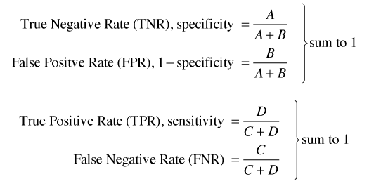
From confusion matrix, Specificity and Sensitivity can be derived as illustrated below:

Specificity and Sensitivity plays a crucial role in deriving ROC curve.

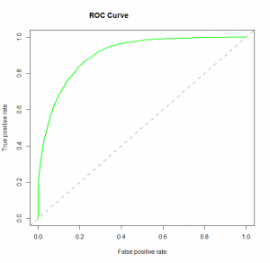
4. ROC Curve: Receiver Operating Characteristic(ROC) summarizes the model’s performance by evaluating the trade offs between true positive rate (sensitivity) and false positive rate(1- specificity). For plotting ROC, it is advisable to assume p > 0.5 since we are more concerned about success rate. ROC summarizes the predictive power for all possible values of p > 0.5.  The area under curve (AUC), referred to as index of accuracy(A) or concordance index, is a perfect performance metric for ROC curve. Higher the area under curve, better the prediction power of the model. Below is a sample ROC curve. The ROC of a perfect predictive model has TP equals 1 and FP equals 0. This curve will touch the top left corner of the graph.

Note: For model performance, you can also consider likelihood function. It is called so, because it selects the coefficient values which maximizes the likelihood of explaining the observed data. It indicates goodness of fit as its value approaches one, and a poor fit of the data as its value approaches zero.

Logistic Regression Model in R and Python

The R code is provided below but if you’re a Python user, here’s an awesome code window to build your logistic regression model. No need to open Jupyter – you can do it all here:

Considering the availability, I’ve built this model on our practice problem – Dressify data set. You can download it here.

Without going deep into feature engineering, here’s the script of simple logistic regression model:

setwd('C:/Users/manish/Desktop/dressdata')

#load data
train <- read.csv('Train_Old.csv')

#create training and validation data from given data
install.packages('caTools')
library(caTools)

set.seed(88)
split <- sample.split(train$Recommended, SplitRatio = 0.75)

#get training and test data
dresstrain <- subset(train, split == TRUE)
dresstest <- subset(train, split == FALSE)

#logistic regression model
model <- glm (Recommended ~ .-ID, data = dresstrain, family = binomial)
summary(model)

predict <- predict(model, type = 'response')

#confusion matrix
table(dresstrain$Recommended, predict > 0.5)

#ROCR Curve
library(ROCR)
ROCRpred <- prediction(predict, dresstrain$Recommended)
ROCRperf <- performance(ROCRpred, 'tpr','fpr')
plot(ROCRperf, colorize = TRUE, text.adj = c(-0.2,1.7))

#plot glm
library(ggplot2)
ggplot(dresstrain, aes(x=Rating, y=Recommended)) + geom_point() + 
stat_smooth(method="glm", family="binomial", se=FALSE)

This data require lots of cleaning and feature engineering. The scope of this article restricted me to keep the example focused on building logistic regression model. This data is available for practice. I’d recommend you to work on this problem. There’s a lot to learn.

End Notes

By now, you would know the science behind logistic regression. I’ve seen many times that people know the use of this algorithm without actually having knowledge about its core concepts. I’ve tried my best to explain this part in simplest possible manner. The example above only shows the skeleton of using logistic regression in R. Before actually approaching to this stage, you must invest your crucial time in feature engineering.

Furthermore, I’d recommend you to work on this problem set. You’d explore things which you might haven’t faced before.

Did I miss out on anything important ? Did you find this article helpful? Please share your opinions / thoughts in the comments section below.

If you like what you just read & want to continue your analytics learning, subscribe to our emails, follow us on twitter or like our facebook page.